Hi,
<div class="text-justify">
In my previous <a href="https://steemit.com/ai/@boostyslf/how-did-i-learn-machine-learning-step-2-setup-conda-environment-in-pycharm">post</a>, I have discussed how to setup conda environment in PyCharm. Today I am going to present to you some key things we need to learn before we implement a neural network and the notations I am going to use in this blog series. By searching the internet also, you can learn these key points. But the reason to explain these things here is that knowledge of these points can be useful to follow my future posts.
###### Structure of a conventional neural network
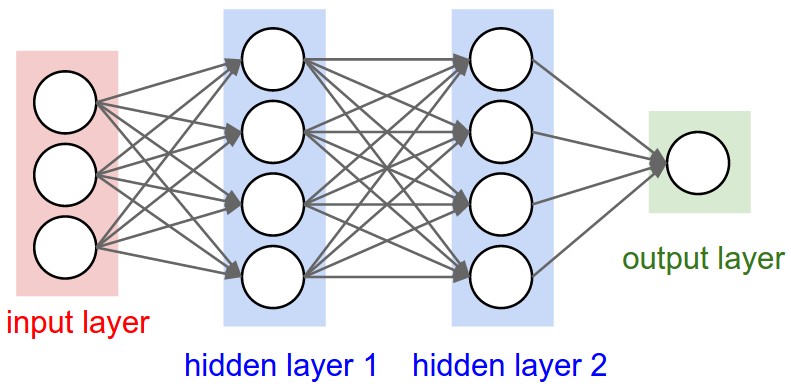
Please refer to the below image to get an idea about a conventional neural network. In a conventional neural network, we can see the input layer, output layer and some number of hidden layers. Each layer has several numbers of neurons. Each neuron is created from the values of the neurons of the previous layer, weight values, and bias value. Also, each layer consists of the activation function and the activation function decides the value which should be pass to the next layer. I will post another blog to explain the functionality of the activation function. If we increase the number of layers and the number of neurons in each layer, the conventional neural network transfers to a deep neural network(dnn). In my future blogs, I will discuss other types of neural networks such as dnn, rnn, etc
###### Forward propagation
We can calculate the values of each layer, by multiplying the weights and values of the previous layer and adding them together. Also, the bias should be added too.
scalar equation:
z<sub>1</sub><sup>(i)</sup> = w<sub>1</sub>x<sub>1</sub><sup>(i)</sup> + w<sub>2</sub>x<sub>2</sub><sup>(i)</sup> + ... + w<sub>n</sub>x<sub>n</sub><sup>(i)</sup> + b
vectorized equation:
Z = WX + B
In the next blog, I will present an example to get more intuition.
###### Cost function
After we calculate the output layer, we should get the cost. Here the cost means the difference between the calculated value(using forward propagation) and actual value. The cost function can vary from a neural network to a neural network.
###### Backward propagation
<div class="pull-left">https://cdn.steemitimages.com/DQmZTrXe3FZSRLenE7UUWDi7TBa9VBwbSzEUHYdzCTe81Z5/cost.png</div>
After we calculate the cost function, we should adjust the cost such the cost should be minimized. For that, we should calculate the derivative of the cost with respect to all weights and bias(∂J/∂w and ∂J/∂b). By using those derivations we can adjust the weights and bias such the cost is minimized.
**w = w - α∂J/∂w
b = b - α∂J/∂b**
This is called the **Gradient Descent**. The gradient of the **point A** is a negative value and the weight should be increased to minimize the cost. Therefore the negative gradient should be subtracted from the weight(w = w - α∂J/∂w). Also, the gradient of the **point B** is a positive value and the weights should be decreased to minimize the cost. Therefore the positive gradient should be subtracted from the weight(w = w - α∂J/∂w). Here **α** denotes the learning rate. The learning rate decides the rate of reducing the cost. I will post a separate blog post to explain the effect of the learning rate.
###### Notations
| Symbol | Explanation |
|-|:-|
|[l]|l th layer|
|{m}|m th mini-batch|
|m|size of the dataset|
|n|number of neurons in one layer|
|simple letter|scalar|
|capital letter|vector|
|(i)|i th sample|
|x<sub>1</sub><sup>(i)</sup>|first input value of the i th sample|
|w<sub>1</sub><sup>[l]</sup>|first weight of the l th layer|
|g()|activation fucntion|
In the next blog, I will explain to you how to implement a neural network by using a real-world example. Please feel free to raise any concerns/suggestions on this blog post. Let's meet in the next post.
</div>