create account

5-18 Iris flowers dataset 적용 Linear Discriminant Analysis I: Histogram 작도 by codingart

View this thread on: hive.blogpeakd.comecency.com
· @codingart · (edited)
$2.59
5-18 Iris flowers dataset 적용 Linear Discriminant Analysis I: Histogram 작도
![noname06.png](https://cdn.steemitimages.com/DQmQFWcL5ine2Dc3wVmU5kAGwengpT4abEsGXStT21G5M5u/noname06.png)

LDA 기법이 오래전에 Fisher  교수에 개발되었지만 자신이 스스로 준비했던 Iris flowers dataset을 사용하여 처리한 자료를 찾기는 어려우므로 직접 파이선 코딩에 의해 풀어 보기로 하자.

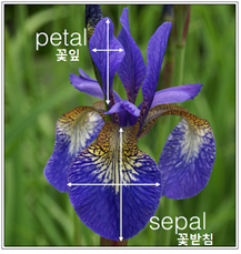
Pandas 의 DataFrame 기법을 사용하여 150개의 데이터를 CSV format으로 읽고 3가지 종류 붓꽃 종들의 컬럼 데이터를 사용하여 빈도수를 막대그래프로 작도해 보자. 붓꽃 데이터의 컬럼 데이터는 4가지 종류로 이루어진다. 즉 꽃받침과 꽃잎의 길이와 폭 데이터들이다. 물론 이 중에 어느 컬럼 데이터를 선택하느냐에 따라 막대그래프 빈도수를 작도해 보면 꽃 종류별로 특정 사이즈 대에서 겹침 현상이 발생한다. 이러한 겹침 현상이 있어도 LDA 기법에 의해 최대한 꽃 종류를 제대로 Classification  할 수 있도록 LDA 기법을 적용해 보기로 한다.

그 일단계로서 붓꽃 데이터베이스로부터 아래 코드에서처럼 다운로드하여 막대그래프 빈도수를 작도해 보도록 하자.

![noname01.png](https://cdn.steemitimages.com/DQmVgvNyaDMi21ZGnuNkDLG6gsyCyahALAUDi8bQJrwsrzw/noname01.png)
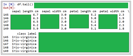
셸(Shell)에서 별도로 df.tail() 명령을 실행하면 아래의 결과를 볼 수 있다.

![noname02.png](https://cdn.steemitimages.com/DQmPcAuUPPPtwAQ4nBaJgH5aDeFuCEcRQisom3iCpqmkbPv/noname02.png)

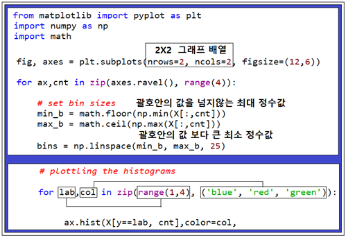
matplotlib 작도 라이브러리를 사용하기 위해서는 데이터들이 리스트형 구조에서 numpy  어레이용으로 변환 처리 되어야 하면 아울러 문자열로 표현된 class를 나타내는 라벨 값들을 숫자 1,2,3 으로 대체하기로 한다.

![noname03.png](https://cdn.steemitimages.com/DQma7EebU3zEQUc71UfLHV8DzPsc5ytW2yhGUvMuHXPcPbk/noname03.png)

막대그래프 구간의 최대 최소값을 정수 형태로 결정한 후 linspace 명령에 의해 구간을 25개 로 나누어 작도하자.

![noname04.png](https://cdn.steemitimages.com/DQmYVZSinbYAGB7XGsto8jGF6Vz3vDe8mFQxhSN7nvDJh5H/noname04.png)

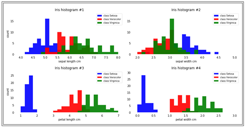
최종적으로 코드를 실행하면 다음과 같은 막대그래프 분포가 얻어진다. 3가지 색상을 제외한 나머지 색상은 2가지 색상의 합성 결과임을 참조하자.
Iris histogram #1과 #2에서는 붓꽃 종간의 겹침이 많음을 볼 수 있다.

![noname05.png](https://cdn.steemitimages.com/DQmbaQEP8NkLthRrqpaD8e1kVrMu3cQLEZFaTAYf4EXhZ8o/noname05.png)

#Iris_lda_01
# -*- coding: utf-8 -*-
"""
Created on Wed May 15 20:43:20 2019
@author: CodingArt
"""
import pandas as pd

s1 = 'sepal length cm'
s2 = 'sepal width cm'
s3 = 'petal length cm'
s4 = 'petal width cm'

feature_dict = {i:label for i,label in zip(range(4),( s1, s2, s3, s4))}

df = pd.io.parsers.read_csv(filepath_or_buffer=
    'https://archive.ics.uci.edu/ml/machine-learning-databases/iris/iris.data',
    header=None,sep=',',)
df.columns = [l for i,l in sorted(feature_dict.items())] + ['class label']
df.dropna(how="all", inplace=True) # to drop the empty line at file-end

df.tail()

from sklearn.preprocessing import LabelEncoder

X=df[[ s1, s2, s3, s4]].values
y = df['class label'].values

enc = LabelEncoder()
label_encoder = enc.fit(y)
y = label_encoder.transform(y) + 1

label_dict = {1: 'Setosa', 2: 'Versicolor', 3:'Virginica'}

from matplotlib import pyplot as plt
import numpy as np
import math

fig, axes = plt.subplots(nrows=2, ncols=2, figsize=(12,6))

for ax,cnt in zip(axes.ravel(), range(4)):  

    # set bin sizes
    min_b = math.floor(np.min(X[:,cnt]))
    max_b = math.ceil(np.max(X[:,cnt]))
    bins = np.linspace(min_b, max_b, 25)

    # plottling the histograms
    for lab,col in zip(range(1,4), ('blue', 'red', 'green')):
        ax.hist(X[y==lab, cnt],color=col,
                   label='class %s' %label_dict[lab],
                   bins=bins,alpha=0.7,)
    ylims = ax.get_ylim()

    # plot annotation
    leg = ax.legend(loc='upper right', fancybox=True, fontsize=8)
    leg.get_frame().set_alpha(0.5)
    ax.set_ylim([0, max(ylims)+2])
    ax.set_xlabel(feature_dict[cnt])
    ax.set_title('Iris histogram #%s' %str(cnt+1))

    # hide axis ticks
    ax.tick_params(axis="both", which="both", bottom="off", top="off",  
            labelbottom="on", left="off", right="off", labelleft="on")

    # remove axis spines
    ax.spines["top"].set_visible(False)  
    ax.spines["right"].set_visible(False)
    ax.spines["bottom"].set_visible(False)
    ax.spines["left"].set_visible(False)    

axes[0][0].set_ylabel('count')
axes[1][0].set_ylabel('count')

fig.tight_layout()       

plt.show()

![마나마인로고.png](https://cdn.steemitimages.com/DQmeePhYx37SUt2zaQJZjJZenWLWSyeK2zKiEp2erB77Lhb/%EB%A7%88%EB%82%98%EB%A7%88%EC%9D%B8%EB%A1%9C%EA%B3%A0.png)
👍  , , , , , , , , , , , , , , , , , , ,
properties (23)
authorcodingart
permlink5-18-iris-flowers-dataset-linear-discriminant-analysis-i-histogram
categorykr
json_metadata{"tags":["kr","kr-new","manamine","weedcash","kr-dev"],"users":["author"],"image":["https://cdn.steemitimages.com/DQmQFWcL5ine2Dc3wVmU5kAGwengpT4abEsGXStT21G5M5u/noname06.png","https://cdn.steemitimages.com/DQmVgvNyaDMi21ZGnuNkDLG6gsyCyahALAUDi8bQJrwsrzw/noname01.png","https://cdn.steemitimages.com/DQmPcAuUPPPtwAQ4nBaJgH5aDeFuCEcRQisom3iCpqmkbPv/noname02.png","https://cdn.steemitimages.com/DQma7EebU3zEQUc71UfLHV8DzPsc5ytW2yhGUvMuHXPcPbk/noname03.png","https://cdn.steemitimages.com/DQmYVZSinbYAGB7XGsto8jGF6Vz3vDe8mFQxhSN7nvDJh5H/noname04.png","https://cdn.steemitimages.com/DQmbaQEP8NkLthRrqpaD8e1kVrMu3cQLEZFaTAYf4EXhZ8o/noname05.png","https://cdn.steemitimages.com/DQmeePhYx37SUt2zaQJZjJZenWLWSyeK2zKiEp2erB77Lhb/%EB%A7%88%EB%82%98%EB%A7%88%EC%9D%B8%EB%A1%9C%EA%B3%A0.png"],"links":["https://archive.ics.uci.edu/ml/machine-learning-databases/iris/iris.data"],"app":"steemit/0.1","format":"markdown"}
created2019-05-18 13:50:51
last_update2019-05-20 05:07:45
depth0
children0
last_payout2019-05-25 13:50:51
cashout_time1969-12-31 23:59:59
total_payout_value1.976 HBD
curator_payout_value0.610 HBD
pending_payout_value0.000 HBD
promoted0.000 HBD
body_length3,820
author_reputation41,833,111,979,966
root_title"5-18 Iris flowers dataset 적용 Linear Discriminant Analysis I: Histogram 작도"
beneficiaries[]
max_accepted_payout1,000,000.000 HBD
percent_hbd10,000
post_id85,083,199
net_rshares4,626,841,211,406
author_curate_reward""
vote details (20)