Most advanced engineering courses feature the resolution of Partial Differential Equations as a relevant topic. This kind of equations led Jean-Baptiste Joseph Fourier to develop his series to solve the Heat equation, the Wave equation is the solution for the Maxwell Equations of Electromagnetism and the Laplace equation is very useful for problems related with Heat and DC potential. Thus, we are in front of one of the most relevant problems for engineering.
In practice, this kind of equation is solved using numerical methods, but for academic aims is important to know how to solve them using analytic steps, for that, we are going to use the Separation of Variables method.
We have solved one exercise and left the other three for your practice, also you will be able to see the graphic solution plotted with Python.
## The problem
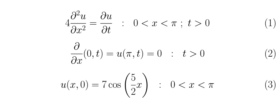
To resolve the heat equation if
## The solution
We have boundary conditions in a finite interval *0 < x < π*, thus we can resolve this equation using the separation of variables, let *u(x,t)=X(x)T(t) ≠ 0* the solution proposed, then we substitute it into *(1)*
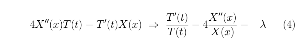
Both parts are equaled to a constant *λ* to impose both independent solutions evolve in time *t* and space *x* at the same rate os change. If we left a member fixed, for instance, the one who depends on *x* and letting the other one change, that will be a mistake, because we would be saying that for all *t* the member that corresponds to the spacial variable doesn't change in time, which is false, the minus sign is only convenience for the math. We extract the following ordinary differential equation from *(4)*

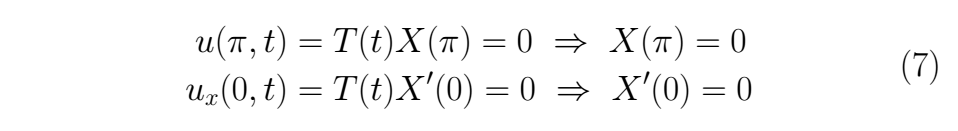
Using the boundary conditions given as data for *u(x,t)* in *(2)* we find the initial condition for the problem in *(5)*, we have to take into account that if *T(t)=0 ; ∀ t* then, we would get a trivial solution for the problem, and we don't want that
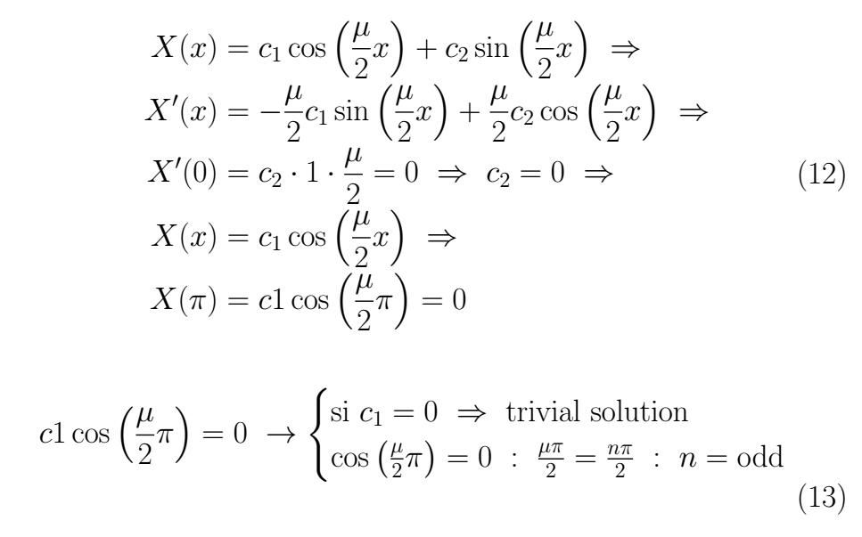
We begin solving for *X(x)*, looking for possibles values to *λ*.
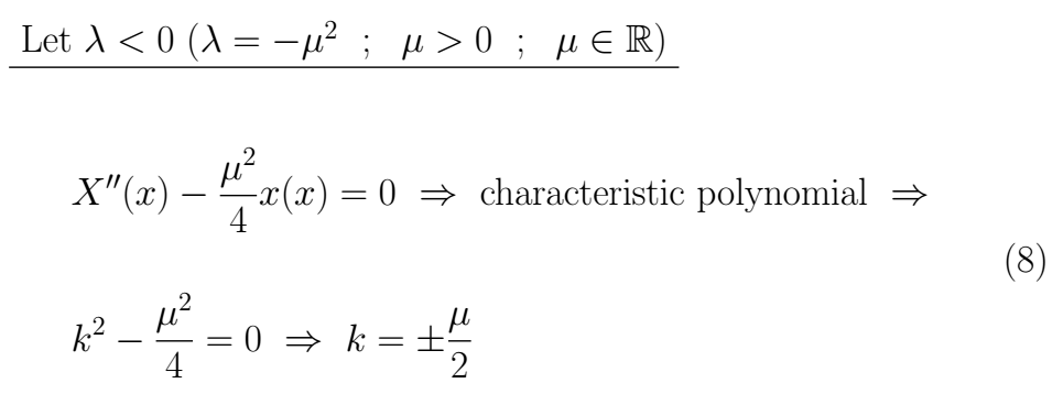
This kind of result leads us towards a linear combination of hyperbolic sines and cosines as a solution.
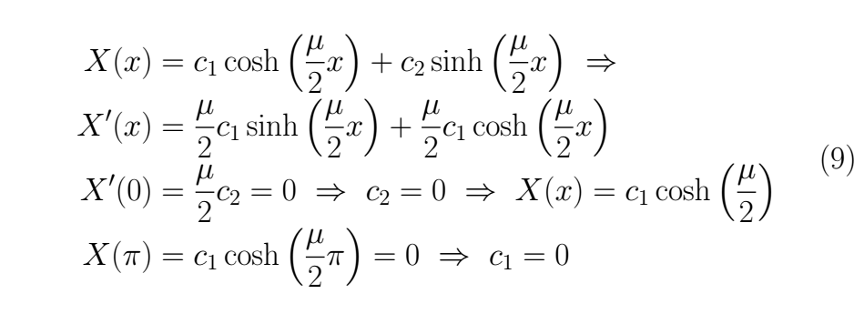
Thus, for *λ < 0* we get as result *X(x)=0* which is a trivial and useless solution.
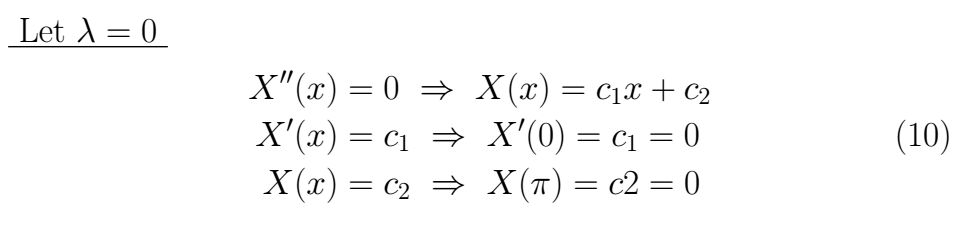
If *λ = 0* we get as result *X(x)=0* which is a trivial and useless solution.
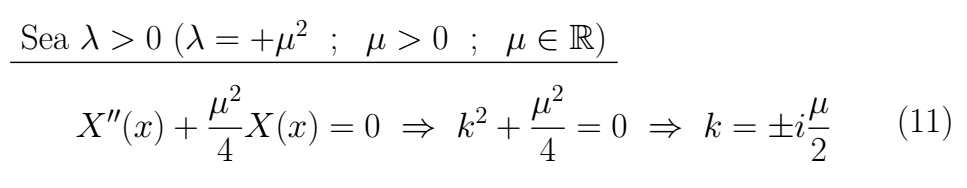
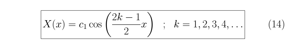
This kind of result leads us towards a linear combination of circular sines and cosines as a solution.
Therefore *μ = (2k-1) ⇒ λ = (2k-1)²*. This give us our first solution
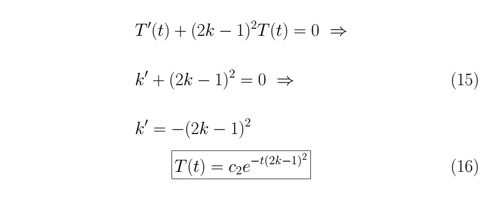
With the *λ* value known we can resolve for *T(t)*.
We assemble the solution
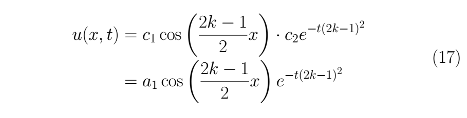
As any linear combination of this kind of solution is also a solution for *(1)*, the expression for the general solution actually is

Now we can use the remainder condition *(3)*
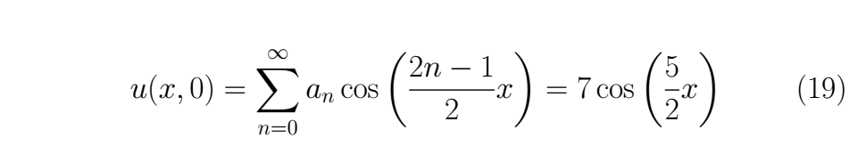
This leads us to develop some terms of the series to find the coefficients that satisfied the equality
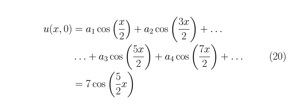
To the past condition can be satisfied, it must necessarily be fulfilled that

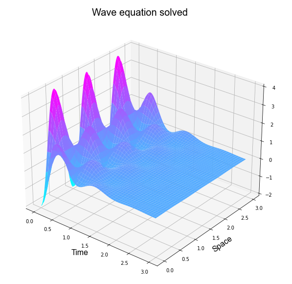
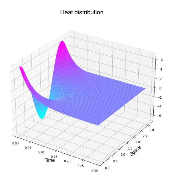
It is possible plotting the past result as
# Other Problems
Let's pose three Partial Differential Equation problems and their result, besides we have included the graphs related to each solution
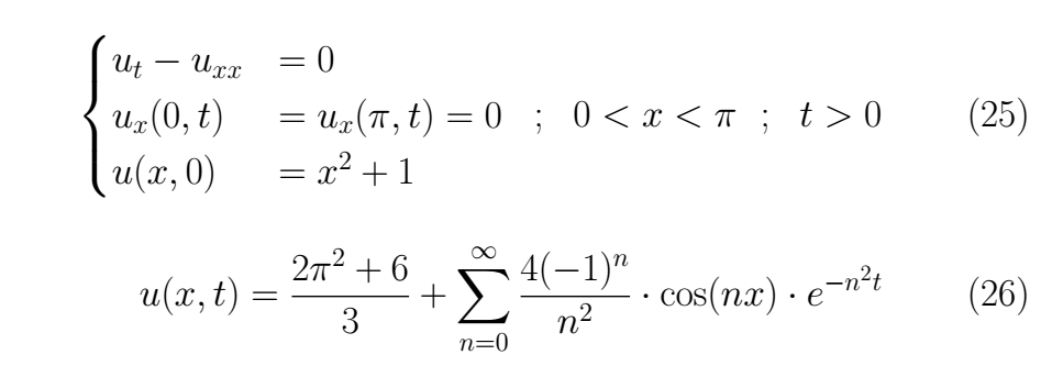
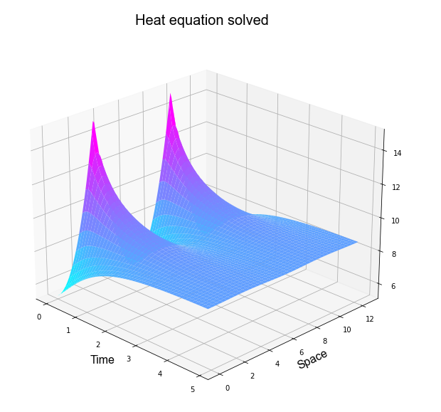
## Problem 1
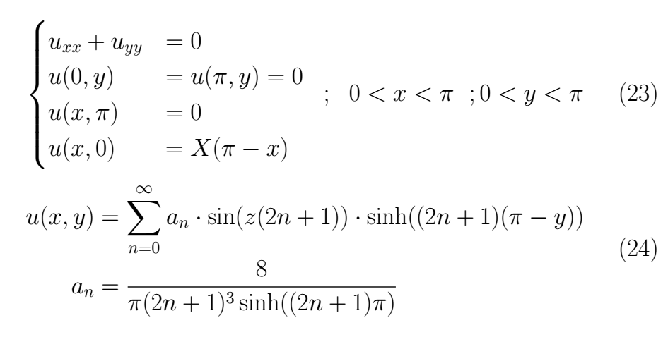
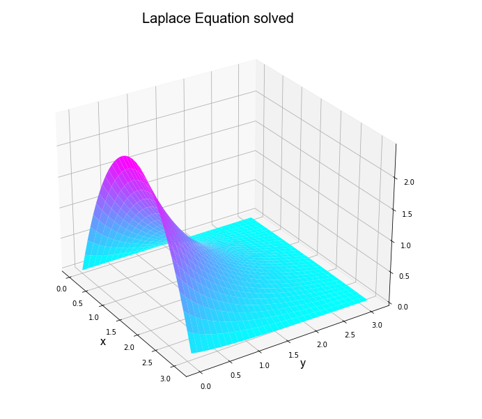
## Problem 2
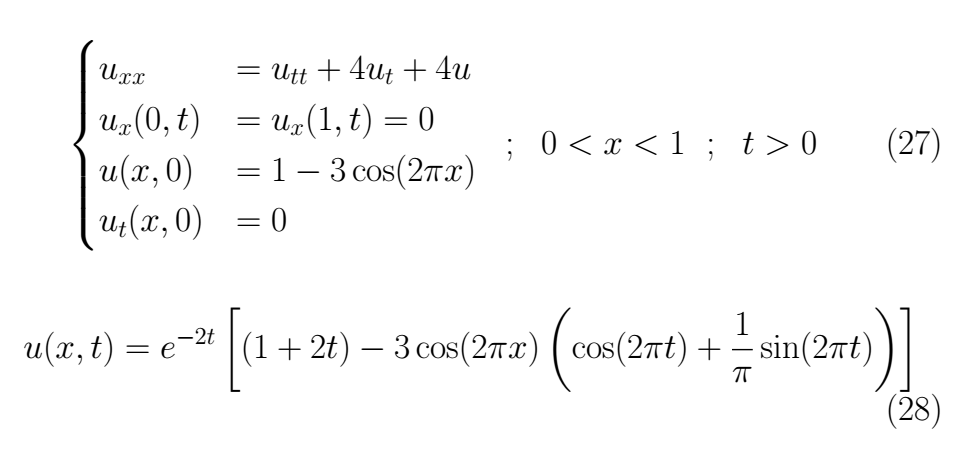
## Problem 3

# Python code for plotting
```
# -*- coding: utf-8 -*-
"""
Created on Thu Aug 13 12:10:44 2020
@author: Venacio
"""
#%%
try:
from IPython import get_ipython
get_ipython().magic('clear') # to clear the terminal
get_ipython().magic('reset -f') # to reset the kernel
get_ipython().magic('matplotlib qt') # plots out line
# get_ipython().magic('matplotlib', 'inline') # plots in line
except:
pass
#%%
import numpy as np
from numpy import *
import sympy as smp
from sympy import *
import matplotlib.pyplot as plt
from matplotlib import cm
from matplotlib.ticker import LinearLocator, FormatStrFormatter
from matplotlib.gridspec import GridSpec
# from mpl_toolkits import mplot3d
import scipy as scp
from scipy.optimize import *
from scipy.integrate import *
import control as co
# import pandas as pd
# import sklearn as sk
# import math
# import os
# import tarfile
# import urllib
np.set_printoptions(precision=4, suppress=True) # number of decimals in the expre.
init_printing(use_unicode=True) # to show in pretty symboic
#%%
x , n = symbols( 'x n' )
T = 2*np.pi
xt = np.arange( -T , T , 1e-2)
xt = np.array([ xt ])
armo = 50
#%%
f1 = (x**4)/24
# f2 = 2 - x
I1 = (x, -pi , pi )
# I2 = (x, 0 , 2 )
a0 = (1/(T))*( integrate( f1 , I1 ) )
a0 = simplify(a0)
an = (2/(T))*( integrate( f1*cos((2*pi/T)*n*x) , I1 ) )
an = simplify(an)
bn = (2/(T))*( integrate( f1*sin((2*pi/T)*n*x) , I1 ) )
bn = simplify(bn)
## Function 1
# a0 = (1/(T))*( integrate( 1 , (x , 0 , T/2) ) +\
# integrate( -1 , (x , T/2 , T) ) )
# a0 = simplify(a0)
# an = (2/(T))*( integrate( 1*cos((2*pi/T)*n*x) , (x , 0 , T/2) ) +\
# integrate( -1*cos((2*pi/T)*n*x) , (x , T/2 , T) ) )
# an = simplify(an)
# bn = (2/(T))*( integrate( 1*sin((2*pi/T)*n*x) , (x , 0 , T/2) ) +\
# integrate( -1*sin((2*pi/T)*n*x) , (x , T/2 , T) ) )
# bn = simplify(bn)
## Function 2
# k, a, b = 64, 1 , 1
# f1 = (a*k/T)*x
# f2 = a
# f3 = (-a*k/T)*(x-T/2)
# f4 = -b
# f5 = (b*k/T)*(x-T)
# I1 = (x, 0, T/k )
# I2 = (x, T/k, (T/2)*((k-2)/k) )
# I3 = (x, (T/2)*((k-2)/k), (T/2)*((k+2)/k) )
# I4 = (x, (T/2)*((k+2)/k), (T)*((k-1)/k) )
# I5 = (x, (T)*((k-1)/k), T )
# a0 = (1/(T))*( integrate( f1 , I1 ) + integrate( f2 , I2 ) +
# integrate( f3 , I3 ) + integrate( f4 , I4 ) +
# integrate( f5 , I5 ) )
# a0 = simplify(a0)
# an = (2/(T))*( integrate( f1*cos((2*pi/T)*n*x) , I1 ) +
# integrate( f2*cos((2*pi/T)*n*x) , I2 ) +
# integrate( f3*cos((2*pi/T)*n*x) , I3 ) +
# integrate( f4*cos((2*pi/T)*n*x) , I4 ) +
# integrate( f5*cos((2*pi/T)*n*x) , I5 ) )
# an = simplify(an)
# bn = (2/(T))*( integrate( f1*sin((2*pi/T)*n*x) , I1 ) +
# integrate( f2*sin((2*pi/T)*n*x) , I2 ) +
# integrate( f3*sin((2*pi/T)*n*x) , I3 ) +
# integrate( f4*sin((2*pi/T)*n*x) , I4 ) +
# integrate( f5*sin((2*pi/T)*n*x) , I5 ) )
# bn = simplify(bn)
## Function 3
# a0 = (1/(T))*( integrate( sin(x) , (x , 0 , T/2) ) +\
# integrate( -sin(x) , (x , T/2 , T) ) )
# a0 = simplify(a0)
# an = (2/(T))*( integrate( sin(x)*cos((2*pi/T)*n*x) , (x , 0 , T/2) ) +\
# integrate( -sin(x)*cos((2*pi/T)*n*x) , (x , T/2 , T) ) )
# an = simplify(an)
# bn = (2/(T))*( integrate( sin(x)*sin((2*pi/T)*n*x) , (x , 0 , T/2) ) +\
# integrate( -sin(x)*sin((2*pi/T)*n*x) , (x , T/2 , T) ) )
# bn = simplify(bn)
#%%
S1, S2 = 0, 0
M1 = np.zeros( (armo , len( xt[0,:] ) ) )
ante = np.zeros( ( 1 , len( xt[0,:] ) ) )
ArC = np.zeros( ( 1 , armo ) )
nArm = np.array( [np.arange( 1 , len(M1[:,0])+1 ) ] )
# Here are created
for N in range( 1 , armo+1 ):
An = float( an.subs( n , N ).evalf() )
Bn = float( bn.subs( n , N ).evalf() )
S1 = An*cos( (2*pi/T)*N*x )
S2 = Bn*sin( (2*pi/T)*N*x )
Lda = lambdify( x , S1 , 'numpy' )
Ldb = lambdify( x , S2 , 'numpy' )
M1[[N-1],:] = ( Lda( xt ) + Ldb( xt ) )
ArC[[0],N-1] = np.max( M1[[N-1],:] )
#%%
# Here are cleaned those harmonics = 0
M1 = np.round( M1 , 4 )
M1 = M1[~np.all(M1 == 0, axis=1)]
nArm2 = np.array( [np.arange( 1 , len(M1[:,0])+1 ) ] )
M2 = np.zeros( M1.shape )
# Here is created a Mtx whose rows are the harmonic sum
for N in range( 1 , len( M2[:,0] ) + 1 ):
if (N == 1):
M2[[N-1],:] = M1[0,:]
if (N > 1):
M2[[N-1],:] = M2[[N-2],:] + M1[[N-1],:]
# The Fourier Series is created
Fourier = a0 + sum(M1 , axis=0)
#%%
fig1 = plt.figure()
ax = fig1.gca( projection='3d' )
surf = ax.plot_surface( nArm2 , xt.T , M2.T ,
linewidth=1,
antialiased=True)
# cmap=cm.coolwarm
# Customize the z axis.
# ax.set_zlim(-1.01, 1.01)
# ax.zaxis.set_major_locator(LinearLocator(10))
# ax.zaxis.set_major_formatter(FormatStrFormatter('%.02f'))
# Add a color bar which maps values to colors.
# fig1.colorbar(surf, shrink=0.5, aspect=5)
plt.show()
#%%
fig1 = plt.figure()
plt.subplot(2,2,(1,2))
plt.plot( xt.T , Fourier.T )
plt.title('Fourier Signal' , fontdict = {'fontname': 'Arial' , 'fontsize':20} )
plt.xlabel('time' , fontdict = {'fontname': 'Arial' , 'fontsize':16} )
plt.ylabel('Signal' , fontdict = {'fontname': 'Arial' , 'fontsize':16} )
plt.subplot(2,2,3)
plt.plot( xt.T , M1.T + a0 )
plt.title('Harmonics' , fontdict = {'fontname': 'Arial' , 'fontsize':20})
plt.xlabel('time' , fontdict = {'fontname': 'Arial' , 'fontsize':16} )
plt.ylabel('Signals' , fontdict = {'fontname': 'Arial' , 'fontsize':16})
plt.subplot(2,2,4)
plt.bar( nArm.reshape(len(nArm[0,:]),) ,
( ArC.reshape(len(ArC[0,:]),) / np.max(M2[0,:]))*100 )
plt.title('Harmonic content' , fontdict = {'fontname': 'Arial' , 'fontsize':20})
plt.xlabel('Harmonics' , fontdict = {'fontname': 'Arial' , 'fontsize':16})
plt.ylabel('Amplitude in % fundamental' , fontdict = {'fontname': 'Arial' , 'fontsize':16})
```