### **I. Introduction**

<center>
![image.png](https://images.hive.blog/DQmSTDUW4WRXz4U8Dyfr9EneNjB48w6iZFasoTaEc1nnmda/image.png)
</center>

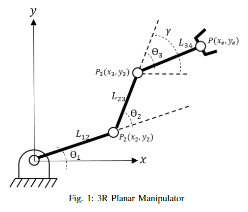
The mathematical modeling of the kinematics of a 3R planar manipulator involved in identifying the end-effector position or the joint angles. The 3R planar manipulator has three revolute joint and three links, as shown in Figure 1. The robot forward kinematics yields the end-effector position and its orientation from the given link lengths and joint angles. On the contrary, the robot inverse kinematics finds the joint angles from the given end-effector and its orientation.

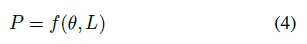
The position of the robot end-effector is denoted by P as

<center>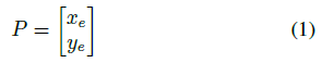![image.png](https://images.hive.blog/DQmZVMGpFyvMr3h2XNJZEPc37ES8o6BxyuM9aT9VxdEmzVz/image.png)</center>

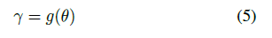
and its orientation relative to the world x-axis is denoted *γ*. The robot joint angles are denoted θ<sub>i</sub>. The trigonometric functions, sine and cosine, are used extensively in the text so the following notations are introduced.

<center>![image.png](https://images.hive.blog/DQmX5MSdeamw58WD69p2wYuQ5NPuGcH4XnHKjQPqMea7dEN/image.png) </center>

This notation is also extended to sums as

<center>![image.png](https://images.hive.blog/DQmNv8jJCyHXz4RkzKRtBnVLCu9nQg8FT2yvAuUmxhtLbsU/image.png)</center>

Link lengths are the distances between the joints and denoted as *L*<sub>ij</sub> , where *i* is the joint number closer to the base and *j* is the joint number to the end-effector. In this text, we derived equations for the forward and inverse kinematics of a 3R planar manipulator, in accordance to the earlier notations. Also, we create *fkinematics* and *ikinematics* functions in MATLAB for forward and inverse kinematics of 3R planar manipulator respectively, and evaluate it by comparing the result of each function.

### **II. METHODS**

#### **A. Forward Kinematics**
The robot forward kinematics calculates the end-effector position and orientation given the joint angles and link lengths. The end-effector position is define by

<center>
![image.png](https://images.hive.blog/DQmePVaWstvAnKkXkDQKKuqipE6psNQJgDBthDeqJF1ZnLF/image.png)
</center>

where θ comprises the joint angles and L is made up of all the link lengths. Also,

<center>
![image.png](https://images.hive.blog/DQmTuYN67A6ENaiEC2qZaQpHoEYNeM1xA2zPzRhzoptBfsq/image.png)
</center>

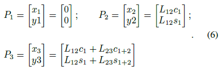
We derived the joint angles using the trigonometric relations in a right triangle. The joint positions are

<center>
![image.png](https://images.hive.blog/DQmX46UUXyiNWjF3a7nAKYswxENX3VecNkBJx8B1UrLp8wB/image.png)
</center>

We take the vector sum of all the joint position and yield the forward kinematic equation for 3R planar manipulator as

<center>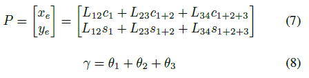![image.png](https://images.hive.blog/DQmRJpMxW8Wwsu84dTag5wEj4P2T2pduASfYFJX1ZXFn1JH/image.png)
</center>

#### **B. Reverse Kinematics**

<center>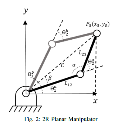![image.png](https://images.hive.blog/DQmbXsR7GaKG6W2jeaJv4LzhNX5SgVNBSP868Jw6RKj4RG7/image.png)
</center>

Robot reverse kinematics is a more useful study because the end-effector position is known. In reverse kinematics problem, the task is to find the joint angles given position *p*, orientation *γ*, and the link lengths. Initially, we solve the position of *P3* and get

<center> 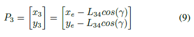![image.png](https://images.hive.blog/DQmTZKu5N8bDqZXQQWc8r6RwKhPd9b9U57k5Te9cx7eBmnR/image.png) </center>

Hence *P3* is obtained by equation 7, the joint angles *θ*<sub>1</sub> and *θ*<sub>2</sub> are given by a 2R inverse kinematics problem with *P3* as the end-effector, as shown in Figure 3. We solve the angles *α* and *β* as

<center>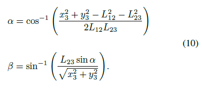![image.png](https://images.hive.blog/DQmazNcSu8q7Uh4sQg7zCgsSYvCBVA2b5YDZZPm4HPNohm5/image.png)</center>

These angles are used to determine the joint angles *θ*<sub>1</sub> and *θ*<sub>2</sub>. We keep in mind that there are two set of solution for the joint angles in 2R inverse kinematics problem. We refer joint 3 as the wrist, and joint 2 as the elbow. We compute the joint angles *θ*<sub>1</sub> and *θ*<sub>2 </sub> by considering the elbow-up and elbow-down configuration, as shown in Figure 2, in reference to wrist angle *θ*<sub>3</sub>.


<center>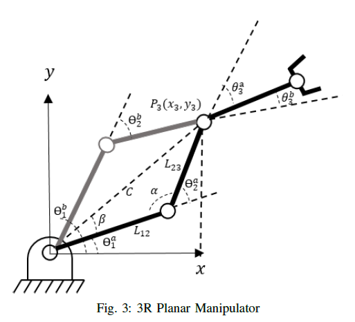![image.png](https://images.hive.blog/DQmXmZNjSWDzJ3J5xsRcHaBMBiZpKXoZYsADwMPAnq2P7Vh/image.png)</center>

The joint angles *θ*<sub>1</sub> and *θ*<sub>2</sub>  are

<center>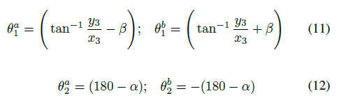![image.png](https://images.hive.blog/DQmQnPfWrZxiK3zHP78oo76NeAmpKDY6Zw7do7odAkaCgzH/image.png)</center>

The wrist angles, *θ*<sub>3</sub>, are

<center>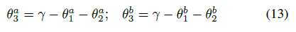![image.png](https://images.hive.blog/DQmUfWtncRniAXjFkYckgc5FjpWhJP9nLunLpwiqkx11EAP/image.png)
</center>

The a and b notation denotes the elbow-up and elbow-down configuration respectively. The joint and wrist angles are shown in Figure 3.

#### **C. MATLAB Implementation**

We implement the equations for the forward and inverse kinematics of a 3R planar manipulator in MATLAB. We create a *fkinematics* and *ikinematics* function for forward and inverse kinematics respectively. The *fkinematics* function accept the link lengths and the joint angles. It returns the end-effector position and orientation. Also, a plot of the 3R planar manipulator and its end-effector point is displayed. The script used for *fkinematics* is shown in listing 1.

```
function fkinematics(links1,links2,links3,theta1,theta2,theta3)
% Forward kinematics for 3-Link Planar Manipulator
% Inputs:
% links1,links2,links3 are length of each links in the robotic arm
% base is the length of base of the robotic arm
% theta1,theta2,theta3 are joint angles in reference to x-axis

format compact
format short

L12 = links1;
L23 = links2;
L34 = links3;
J1 = theta1;
J2 = theta2;
J3 = theta3;

%joint equation
x2 = L12*cosd(J1);
x3 = L23*cosd(J1+J2)+ x2;
xe = L34*cosd(J1+J2+J3) + x3;
y2 = L12*sind(J1);
y3 = L23*sind(J1+J2)+ y2;
ye = L34*sind(J1+J2+J3) + y3;
gamma = J1+J2+J3;
fprintf('The position of the end-effector is (%f, %f) and orientation is(%f)\n',xe,ye,gamma)

%plotting the links
r = L12 + L23 + L34;
daspect([1,1,1])
rectangle('Position',[-r,-r,2*r,2*r],'Curvature',[1,1],...
    'LineStyle',':')
hold on
axis([-r r -r r])
line([0 x2], [0 y2])
line([x2 x3],[y2 y3])
line([x3 xe],[y3 ye])
line([0 0], [-r/10 r/10], 'Color', 'r')
line([-r/10 r/10], [0 0], 'Color', 'r')
hold on
plot([0 x2 x3],[0 y2 y3],'o')
plot([xe],[ye],'o','Color','r')
grid on
xlabel('x-axis')
ylabel('y-axis')
title('Forward Kinematics 3-Link Planar Manipulator')
end
```
<center>Listing 1: Forward Kinematics implementation (fkinematics function)</center>

We set the link lengths, the end-effector position, and orientation as the input for the *ikinematics* function.  The function returns the joint angles and a plot showing the 3R planar manipulator. Hence the inverse cosine yields to either a real or complex value, we set a conditional statement in the script so that inverse cosine would return a real-valued angle. The script used for *ikinematics* is shown in listing 2.

```
function ikinematics(links1, links2, links3, positionx, positiony, gamma)
% Inverse kinematics for 3-Link Planar Manipulator
% Inputs:
% links1,links2,links3 are length of each links in the robotic arm
% base is the length of base of the robotic arm
% positionx,positiony are joint angles in reference to x-axis
% gamma is the orientation

format compact
format short

L12 = links1;
L23 = links2;
L34 = links3;
xe = positionx;
ye = positiony;
g = gamma;

%position P3
x3 = xe-(L34*cosd(g));
y3 = ye-(L34*sind(g));
C = sqrt(x3^2 + y3^2);

if (L12+L23) > C
    %angle a and B
    a = acosd((L12^2 + L23^2 - C^2 )/(2*L12*L23));
    B = acosd((L12^2 + C^2 - L23^2 )/(2*L12*C));

    %joint angles elbow-down
    J1a = atan2d(y3,x3)-B;
    J2a = 180-a;
    J3a = g - J1a -J2a;

    %joint angles elbow-up
    J1b = atan2d(y3,x3)+B;
    J2b = -(180-a);
    J3b = g - J1b - J2b;

    fprintf('The joint 1, 2 and 3 angles are (%f,%f, %f) respectively for elbow-down configuration.\n',J1a,J2a,J3a)
    fprintf('The joint 1, 2 and 3 angles are (%f,%f, %f) respectively for elbow-up configuration.\n',J1b,J2b,J3b)
else 
    disp('     Dimension error!')
    disp('     End-effecter is outside the workspace.')
    return
end
x2a = L12*cosd(J1a);
y2a = L12*sind(J1a);
x2b = L12*cosd(J1b);
y2b = L12*sind(J1b);
r = L12 + L23 + L34;
daspect([1,1,1])
rectangle('Position',[-r,-r,2*r,2*r],'Curvature',[1,1],...
    'LineStyle',':')
line([0 x2a], [0 y2a],'Color','b')
line([x2a x3], [y2a y3],'Color','b')
line([x3 xe], [y3 ye],'Color','b')
line([0 x2b], [0 y2b],'Color','g','LineStyle','--')
line([x2b x3], [y2b y3],'Color','g','LineStyle','--')
line([x3 xe], [y3 ye],'Color','b','LineStyle','--')
%line([0 xe], [0 ye],'Color','r')
line([0 0], [-r/10 r/10], 'Color', 'r')
line([-r/10 r/10], [0 0], 'Color', 'r')
hold on
plot([0 x2a x3],[0 y2a y3],'o','Color','b')
plot([x2b],[y2b],'o','Color','g')
plot([xe],[ye],'o', 'Color', 'r')
grid on
xlabel('x-axis')
ylabel('y-axis')
title('Inverse Kinematics 3-Links Planar Manipulator')
end
```
<center>Listing 2: Inverse Kinematics implementation (ikinematics function)</center>

### **III. Result and Discussion**

<center>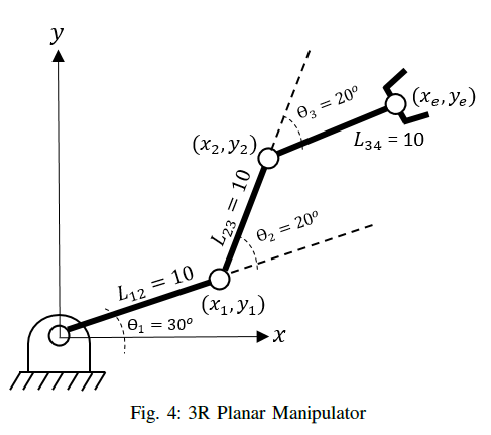![image.png](https://images.hive.blog/DQmd7eRzMSBwP3VgE6XpMv8LSg889N8VnSbDNYSQoRRrFDT/image.png)</center>

#### *A. Forward Kinematics*
In this section, we evaluate the forward and inverse kinematics equations of a 3R planar manipulator. We substitute the values shown in Figure 4 in the fkinematics. In the Matlab window console, we run

```
fkinematics(10,10,10,30,20,20)
```

and yield to the end-effector position, *(x*<sub>e</sub> *= 18.508332, y*<sub>e</sub> *= 22.057371)* and orientation, *(γ = 70.00)*. Figure 5 shows the 3R planar manipulator.

<center>![image.png](https://images.hive.blog/DQmeBvEnBq5ysNzXXisibELBK6oJukhm84brZaM2RWHPpP4/image.png)
</center>

The end-effector position and its orientation from the *fkinematics* is set as an input to  *ikinematics* to evaluate it. The function must yield the joint angles shown in Figure 4. We run

```
ikinematics(10,10,10,18.508332,22.057371,70)
```

and we yield the following joint angles for elbow-down configuration are *θ*<sub>1</sub> *= 30.000009*, *θ*<sub>2</sub> *= 19.999981*, and *θ*<sub>3</sub> *= 20.000009*. Hence the inverse kinematics has two set of unique solution, we have the joint angles for elbow-up configuration as *θ*<sub>1</sub> *= 49.999991*, *θ*<sub>2</sub> *= −19.999981*, and *θ*<sub>3</sub> *= 39.999991*.

<center>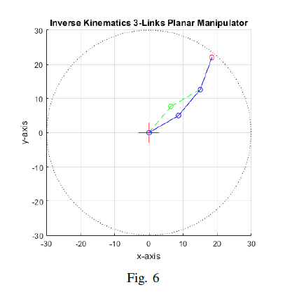![image.png](https://images.hive.blog/DQmYcVikCHF5Zbba6NBuaeqMGLaJeyuBct31bsCsaZNoLb7/image.png)
</center>

Thus, we verified that the forward kinematics equations which yields to a correct end-effector position and its orientation.

<center>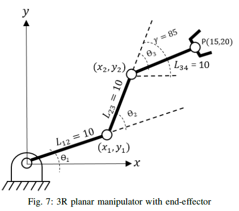![image.png](https://images.hive.blog/DQmf4nM6G5eM1JTGHDs87V93D7uk2ccsypyRpCkvMpFSHRW/image.png)</center>

#### **B. Inverse Kinematics**
Figure 7 shows a 3R planar manipulator with an identified end-effector position and its orientation. We use *ikinematics* function in MATLAB to generate the joint angles. Then, we evaluate the result by substituting it as an input to *fkinematics* function. In the Matlab window console, we run

```
 ikinematics(10,10,10,15,20,85)
```

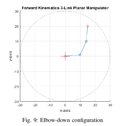
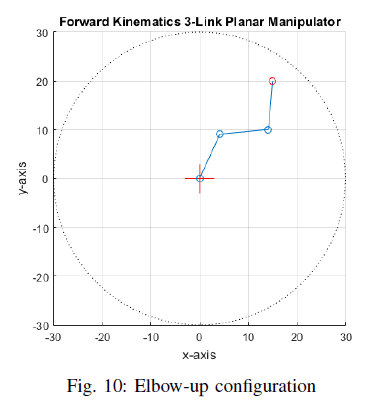
and yield a joint angle for elbow-down configuration as *θ*<sub>1</sub> *= 5.455370, θ* <sub>2</sub> *= 59.875741, θ*<sub>3</sub> *= 19.668889* while for elbow-up configuration as *θ*<sub>1</sub> *= 65.331111, θ*<sub>2</sub> *= −59.875741, θ*<sub>3</sub> *= 79.544630*. Figure 9 shows the 3R planar manipulator plot for the end-effector position *x*<sub>e</sub> *= 15*, *y*<sub>e</sub> *= 20* and its orientation, *γ = 85*. 

<center>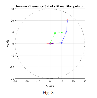![image.png](https://images.hive.blog/DQmRtmgkXBXXAydACjsFzWdBKA8PBviSgzksk3mUSDejYaK/image.png)
</center>

We validate the result by substituting the values to *fkinematics* and in Matlab console, run

```
 fkinematics(10,10,10,5.455,59.876,19.669)
```

This gives us an end-effector position equal to *x*<sub>e</sub> *= 15.000024* and *y*<sub>e </sub> *= 19.999928*, and orientation equal to *γ = 85*. The joint angles in elbow-up configuration also yield to the same end-effector and orientation.


<center>
![image.png](https://images.hive.blog/DQmeh2yG2FEiCTv5jvyHn9xFfHBTLk2oNUnM76y2TS1xe6q/image.png)
</center>

<center>
![image.png](https://images.hive.blog/DQmc7rAAMd9H4mgHCjok1SvipzDBCehkJGfBTJ8pwgpKWyD/image.png)
</center>

Thus, we verified that the inverse kinematics equations which yields to the joint angles.

### **IV. Conclusion**

In this text, we modelled the equations for the forward and inverse kinematics of a 3R planar manipulator as shown in Figure 1. In MATLAB, we wrote a script for the *fkinematics* and *fkinematics* functions. These functions are used to validate the forward and invers kinematics model in the text. The *fkinematics* function returns the end-effector position *P* and its orientation *γ*. The result of fkinematics is validate by using its result as an input to ikinematics function. On the contrary, the ikinematics function returns the join angles θ<sub>1</sub>, θ<sub>2</sub> and θ<sub>3</sub>. We cross-validate the joint angles by setting it as an input to the fkinematic function.

Thus, the forward and inverse kinematics model yield to correct values for the end-effector position and its orientation, and the joint angles. Also, the joint angles, either elbow-up and elbow-down configuration, in the inverse kinematics model gives the same end-effector point and orientation when cross-validated.

### **V. References**

[1] [Lynch, K. and F. Park. “Modern Robotics: Mechanics, Planning, and Control.” (2017).](https://www.semanticscholar.org/paper/Modern-Robotics%3A-Mechanics%2C-Planning%2C-and-Control-Lynch-Park/ad094b63ac4c75239a5ea4464ecc79e73efd2fcd)

[2] [John J. Craig. 1989. Introduction to Robotics: Mechanics and Control (2nd. ed.). Addison-Wesley Longman Publishing Co., Inc., USA.](http://www.mech.sharif.ir/c/document_library/get_file?uuid=5a4bb247-1430-4e46-942c-d692dead831f&groupId=14040)

[3] [Merat, Frank. (1987). Introduction to robotics: Mechanics and control. Robotics and Automation, IEEE Journal of. 3. 166 - 166. 10.1109/JRA.1987.1087086](https://www.researchgate.net/publication/224729839_Introduction_to_robotics_Mechanics_and_control)

(Note: All images in the text are personally drawn by the author except those with citations. )

Posted with [STEMGeeks](https://stemgeeks.net)

Posted with [STEMGeeks](https://stemgeeks.net)