<div class="pull-left"><h1>A</h1></div> <br> lright! <br>So, we saw how to perform <b>Linear Regression</b> and <b>Polynomial Regression</b> (using a quadratic polynomial) in the first part to this two part series!
>**NOTE:** If you haven't seen the previous post, you can read it here: [Predicting Hive - An Intro to Regression - 1](https://peakd.com/@medro-martin/...).
> **NOTE:** Obtaining a better prediction only means that we have higher chances of being closer to the actual value when the event happens in reality.
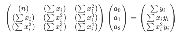
## 1) Polynomial Regression (order 2) - Revisited
In order to use a quadratic, equation, the matrix equation that needs to be solved is as follows:
https://files.peakd.com/file/peakd-hive/medro-martin/N0YirkmC-image.png
The code that we wrote for this kind of regression was:
```
import os
import numpy as np
import matplotlib.pyplot as plt
# Function to sum the elements of an array
def sum(a):
sum = 0
for i in range(len(a)):
sum += a[i]
return sum
fileData = open("<location>/data.csv", "r")
for line in fileData:
line = fileData.readlines()
print(*line)
x = np.zeros(len(line))
y = np.zeros(len(line))
for i in range(len(line)):
x[i], y[i]= line[i].split(",")
sumX = sum(x)
sumX2 = sum(pow(x,2))
sumX3 = sum(pow(x,3))
sumX4 = sum(pow(x,4))
sumY = sum(y)
sumXY = sum(x*y)
sumX2Y = sum(pow(x,2)*y)
print(x,y)
print("sumX, sumX2, sumX3, sumX4, sumY, sumXY, sumX2Y", sumX, sumX2, sumX3, sumX4, sumY, sumXY, sumX2Y)
n = 3
data_m = np.zeros((n,n+1))
#Explicitly Defining the Augmented Matrix
data_m[0,0] = n
data_m[0,1] = sumX
data_m[0,2] = sumX2
data_m[0,3] = sumY
data_m[1,0] = sumX
data_m[1,1] = sumX2
data_m[1,2] = sumX3
data_m[1,3] = sumXY
data_m[2,0] = sumX2
data_m[2,1] = sumX3
data_m[2,2] = sumX4
data_m[2,3] = sumX2Y
print("Initial augmented matrix = \n", data_m)
# Elimination
for j in range(1,n):
#print("LOOP-j:", j)
for k in range(j,n):
#print(" LOOP-k:", k)
factor = data_m[k,j-1] / data_m[j-1,j-1]
for i in range(n+1):
#print(" LOOP-i:", i, "| ", data_m[k,i])
data_m[k,i] = format(data_m[k,i] - factor*data_m[j-1,i], '7.2f')
#print("-->",data_m[k,i])
print("Matrix after elimination = \n", data_m)
# Back Substitution
solution = np.zeros(n)
for j in range(n-1, -1, -1):
subtractant = 0
for i in range(n-1,-1,-1):
subtractant = subtractant + solution[i] * data_m[j,i]
solution[j] = (data_m[j,n] - subtractant)/data_m[j,j]
print("Solution matrix:\n", solution)
y2 = solution[0] + solution[1]*x + solution[2]*pow(x,2)
ax = plt.subplot()
ax.plot(28*x,y, "ob", linestyle="solid")
ax.plot(28*x, y2, "ob", linestyle="solid", color="g")
ax.plot(350,(solution[0] + solution[1]*12.5 + solution[2]*pow(12.5,2)), 'ro')
plt.grid(True)
plt.title("Hive Price Chart")
ax.set_xlabel("Time (days)")
ax.set_ylabel("Price in USD")
plt.show()
```
...and the output we got looked something like this:
|||
|---|---|
|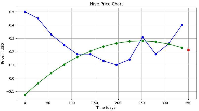|The green curve is the one we have fitted, the blue one is the actual data, and the red dot is our prediction for June 1.|
Now, we'll try to improve our curve-fitting and try to use a Polynomial Regression using higher order polynomial, so that we can get a more accurate prediction.
## 2) Why do we need higher order polynomials?
Just ponder upon the following statements:
- A unique curve that'll always pass through **two** given points is a **straight line**.
- A unique curve that'll pass through three given points is a quadratic polynomial.
- ...and so on...
- **A unique curve that'll pass through n given points is a polynomial of order (n-1).**
That's the reason behind our craving for an n-th order poly.
If we take the matrix equation for the previous quadratic case and carefully look at it, we'll find a pattern...
(Just have a look again!)
> **PATTERN:**
>- In the first matrix, we can clearly see how the powers of `xi` keep increasing as we move down and to the right. This matrix is actually symmetric about its diagonal.
>- Next, in the matrix **P** (i.e. the right-most one), we again have powers of `xi` progressively increasing as we move down.
So, building upon the pattern, we can easily say that the matrix equation to be solved for n<sup>th</sup> order polynomial will be:
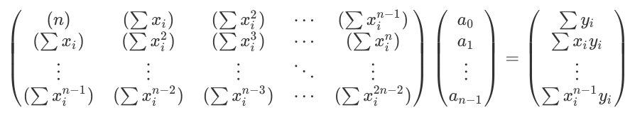
Now, based upon our knowledge, we'll modify the code for the quadratic case, and make it generalised.
**Full Code:**
```
import os
import numpy as np
import matplotlib.pyplot as plt
# Function to sum the elements of an array
def sum(a):
sum = 0
for i in range(len(a)):
sum += a[i]
return sum
fileData = open("<location>/data.csv", "r")
for line in fileData:
line = fileData.readlines()
print("Data received:\n",*line)
x = np.zeros(len(line))
y = np.zeros(len(line))
for i in range(len(line)):
x[i], y[i]= line[i].split(",")
print("x-matrix:\n",x,"\n y-matrix:\n",y)
# Defining order for the polynomial to be used in regression
order = input("Please enter the order of the polynomial you wish to use for interpolation.")
if (order == "default"):
n = len(x)
if (order != "default"):
n = int(order) + 1
print(n, type(n))
data_m = np.zeros((n,n+1))
#Explicitly Defining the Augmented Matrix
#Generalising Augmented Matrix Definition
# Defining the matrix A
for j in range(0,n): #Row counter
for i in range(0,n): #Column counter
if(i == 0 and j == 0):
data_m[j,i] = n
if(i!=0 or j!=0):
data_m[j,i] = sum(pow(x,(i+j)))
# Defining the matrix B
for j in range(0,n):
data_m[j,n] = sum(y*pow(x,j))
print("Initial augmented matrix = \n", data_m)
# Elimination
for j in range(1,n):
#print("LOOP-j:", j)
for k in range(j,n):
#print(" LOOP-k:", k)
factor = data_m[k,j-1] / data_m[j-1,j-1]
for i in range(n+1):
#print(" LOOP-i:", i, "| ", data_m[k,i])
data_m[k,i] = format(data_m[k,i] - factor*data_m[j-1,i], '7.2f')
#print("-->",data_m[k,i])
print("Matrix after elimination = \n", data_m)
# Back Substitution
solution = np.zeros(n)
for j in range(n-1, -1, -1):
subtractant = 0
for i in range(n-1,-1,-1):
subtractant = subtractant + solution[i] * data_m[j,i]
solution[j] = (data_m[j,n] - subtractant)/data_m[j,j]
print("Solution matrix:\n", solution)
y2 = np.zeros(len(x))
for j in range(0,n):
y2 = y2 + solution[j]*pow(x,j)
print(y2)
ax = plt.subplot()
ax.plot(28*x,y, "ob", linestyle="solid")
ax.plot(28*x, y2, "ob", linestyle="solid", color="g")
plt.grid(True)
plt.title("Hive Price Chart")
ax.set_xlabel("Time (days)")
ax.set_ylabel("Price in USD")
plt.show()
```
> **Additional Features we have added:**
>- The user can now decide the order of the polynomial to fit. Selecting `default` tells the program to take the total number of data points as the order of the polynomial.
One thing we haven't added yet is the prediction (extrapolation) part. We need to extrapolate the fitted curve to `day=350`, to get the Hive price on June 1 2020.
For this, we'll just make the following changes near the end of code just above `plt.show()` :
```
.
.
.
for j in range(0,n):
y2 = y2 + solution[j]*pow(x,j)
def predict(x):
prediction = 0
for j in range(0,n):
prediction += solution[j]*pow(x,j)
return prediction
print(y2)
ax = plt.subplot()
ax.plot(28*x,y, "ob", linestyle="solid")
ax.plot(28*x, y2, "ob", linestyle="solid", color="g")
ax.plot(350,predict(12.5), 'ro')
plt.grid(True)
plt.title("Hive Price Chart")
ax.set_xlabel("Time (days)")
ax.set_ylabel("Price in USD")
.
.
.
```
> **NOTE:** As already mentioned in the previous post, we are using `12.5` and not `350` for our prediction because our step size is 28. (12.5 * 28 = 350).
Now, our coding part is complete!...and we are **ready to test and predict**!!
|**Order of Polynomial** | **Fit** | **Prediction**|
|---|---|---|
|1 (linear)|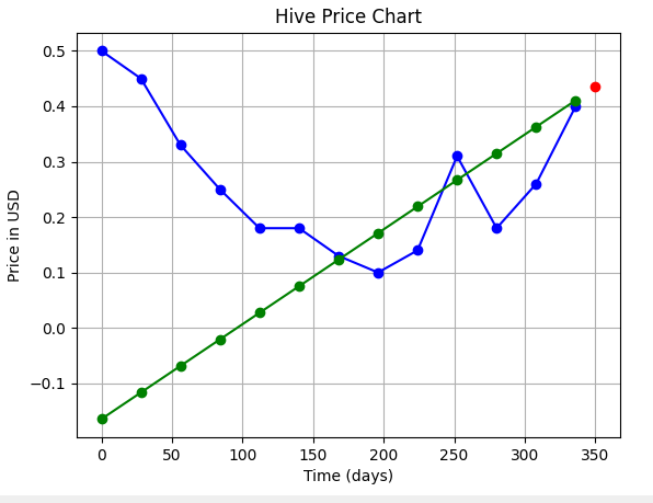|**0.043 $** (ERROR: Here, one thing is very clear. This fit shouldn't start from 0!)|
|2 (quadratic)|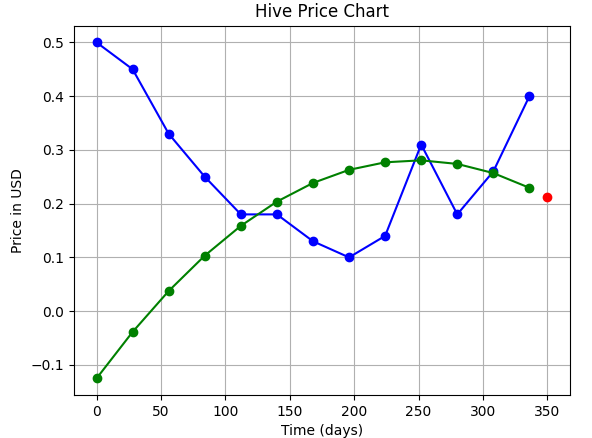|**0.214 $**|
|3 (cubic)|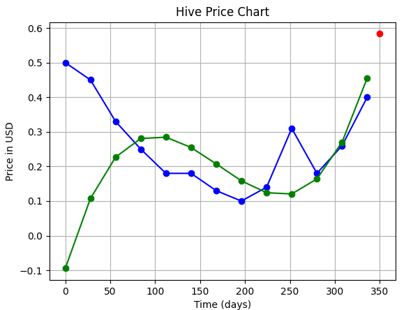|**0.58 $**|
|4|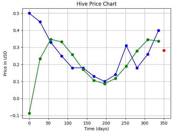|**0.28 $**|
|10|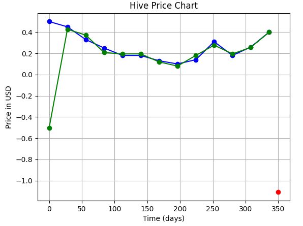|**-1.103 $** (The ERROR is very much clear here!!)|
|default (order = 12)|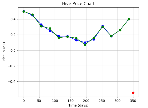|**-0.55 $** (Haha!!)|
Ok, so we have seen above that though polynomial interpolation seems to fit the data well..but, we have checked at intervals of `x = 28`...let's try checking the fitted function at a higher resolution so that we can see what is happening in between those points.
> **Plus we also know one problem with this technique, that the curves always try to pass from near 0 before they rise up to the desired level.**
In the table above, we can see the curve clearly up till an order of 4, but for higher orders, the curve is not clear because of the low resolution we have used to print it. So, let's use higher resolution, and see how the curve really performs...this will also tell us why we are getting odd, erroneous predictions.
|**Order of Polynomial**|**Fit**|**Comments**|
|---|---|---|
|5|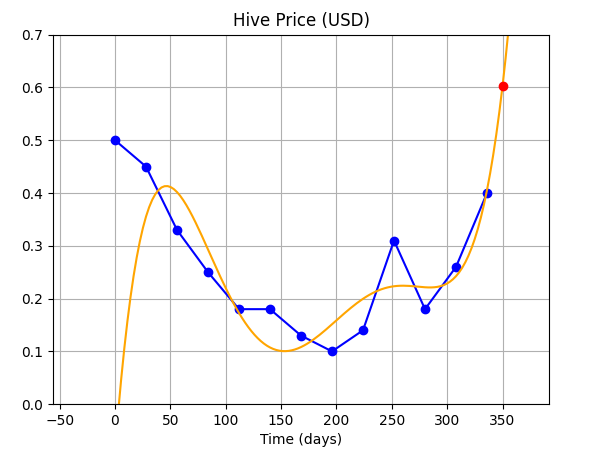|We can see the curve varies wildly between data points.|
|8|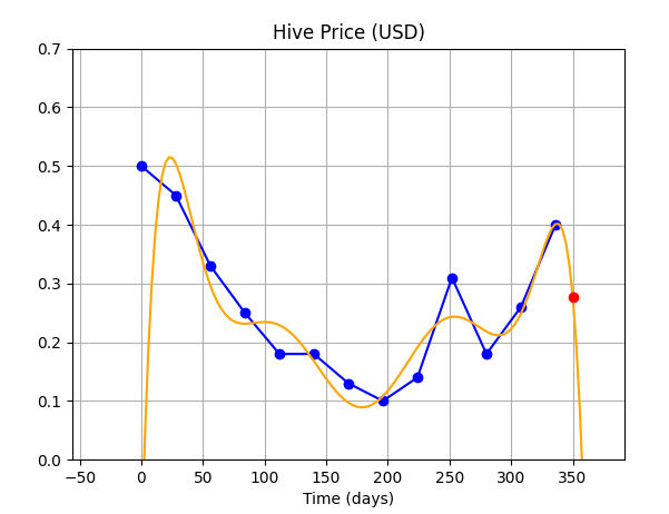||
|10|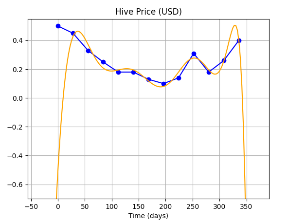|This choice of order performs the worst (for our case).|
|14|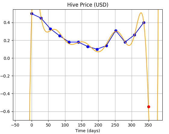||
**So, as you can see...using higher order polynomials to fit the curve is not much of a boon because it gives the curve, extra degrees of freedom, allowing the curve to vary wildly between and beyond the given data points.**
**CONCLUSION:** Using Higher order polynomials may be good for fitting the data, but it is definitely not a good idea for use in extrapolation, and for purposes of prediction.
**IN THE NEXT ARTICLE:**
We'll see how to find the optimum order of polynomial to fit our curve, too low is bad because it doesn't fit the data properly, and hence has less amount of info, too high is also bad because it allows the curve to vary wildly. **Optimisation is the key!!**
---
Hope you learned something new from this article!
Thanks for your time.
Best,
M. Medro
---
#### Credits
All media used in this article have been created by me.| author | medro-martin |
|---|---|
| permlink | predicting-hive-an-intro-to-regression-2 |
| category | hive-196387 |
| json_metadata | {"app":"peakd/2020.05.5","format":"markdown","tags":["steemstem","science","maths","programming","python","coding","regression","hive","hive-148441"],"users":["medro-martin"],"links":["/@medro-martin/..."],"image":["https://files.peakd.com/file/peakd-hive/medro-martin/N0YirkmC-image.png","https://images.hive.blog/p/MG5aEqKFcQi6ksuzVh6JJptBJCL6eFwx2gvRnpcRhTRKgmTKc5WMfwDzRmfFiVA4JeJuTt9JwqPfGcaadwxKy5JaHz9tgwDin?format=match&mode=fit","https://images.hive.blog/p/MG5aEqKFcQi6ksuzVh6JJptBJCL6eFwx2gvRnpcRhTRKgmTKc5WMfwDzRmfFiVA4JeJuTt9JvWEMQZHS2iWnz66ZrAbsxrSxN?format=match&mode=fit","https://files.peakd.com/file/peakd-hive/medro-martin/xuz8HuJ2-image.png","https://files.peakd.com/file/peakd-hive/medro-martin/HrCCCOAA-image.png","https://files.peakd.com/file/peakd-hive/medro-martin/z830TTZv-image.png","https://files.peakd.com/file/peakd-hive/medro-martin/OtIernQr-image.png","https://files.peakd.com/file/peakd-hive/medro-martin/GWDEeYsn-image.png","https://files.peakd.com/file/peakd-hive/medro-martin/aWSkUlgI-image.png","https://files.peakd.com/file/peakd-hive/medro-martin/HPNrYxem-image.png","https://files.peakd.com/file/peakd-hive/medro-martin/vXmaPC1p-image.png","https://files.peakd.com/file/peakd-hive/medro-martin/RREaEoPs-image.png","https://files.peakd.com/file/peakd-hive/medro-martin/1quVNbkd-image.png","https://files.peakd.com/file/peakd-hive/medro-martin/hU7QW90H-image.png"]} |
| created | 2020-06-04 05:15:42 |
| last_update | 2020-06-04 17:51:42 |
| depth | 0 |
| children | 4 |
| last_payout | 2020-06-11 05:15:42 |
| cashout_time | 1969-12-31 23:59:59 |
| total_payout_value | 10.360 HBD |
| curator_payout_value | 10.102 HBD |
| pending_payout_value | 0.000 HBD |
| promoted | 0.000 HBD |
| body_length | 11,201 |
| author_reputation | 12,784,697,208,436 |
| root_title | "Predicting Hive - An Intro to Regression - 2" |
| beneficiaries | [] |
| max_accepted_payout | 1,000,000.000 HBD |
| percent_hbd | 10,000 |
| post_id | 97,763,198 |
| net_rshares | 41,727,278,708,157 |
| author_curate_reward | "" |
| voter | weight | wgt% | rshares | pct | time |
|---|---|---|---|---|---|
| tombstone | 0 | 112,087,258,073 | 2.34% | ||
| simba | 0 | 2,609,497,032 | 4.22% | ||
| tuck-fheman | 0 | 900,850,275 | 4.22% | ||
| drifter1 | 0 | 1,504,356,095 | 4.22% | ||
| chris4210 | 0 | 37,736,505,715 | 4.22% | ||
| eeks | 0 | 5,180,872,516,001 | 100% | ||
| kevinwong | 0 | 1,095,596,154,636 | 13% | ||
| scalextrix | 0 | 1,578,998,529 | 4.22% | ||
| justtryme90 | 0 | 249,790,210,255 | 65% | ||
| eric-boucher | 0 | 17,860,136,656 | 4.22% | ||
| thecryptodrive | 0 | 2,868,822,152 | 1.69% | ||
| mangou007 | 0 | 8,511,442,367 | 5.5% | ||
| anwenbaumeister | 0 | 388,789,782 | 8.44% | ||
| grandpere | 0 | 3,446,573,691 | 100% | ||
| mammasitta | 0 | 544,092,569 | 0.1% | ||
| skapaneas | 0 | 34,443,242,680 | 19.5% | ||
| gerber | 0 | 167,632,728,327 | 2.4% | ||
| roelandp | 0 | 830,280,618,575 | 32.5% | ||
| daan | 0 | 58,146,281,336 | 8% | ||
| ezzy | 0 | 188,391,020,157 | 2.4% | ||
| matt-a | 0 | 664,339,369 | 1.5% | ||
| mrwang | 0 | 4,273,208,625 | 6.5% | ||
| asim | 0 | 1,003,402,835 | 4.22% | ||
| diana.catherine | 0 | 1,042,823,688 | 4.22% | ||
| arcange | 0 | 99,811,277,465 | 3% | ||
| blueorgy | 0 | 2,506,916,814 | 6.33% | ||
| exyle | 0 | 232,420,299,913 | 2.4% | ||
| arconite | 0 | 4,630,823,906 | 6.5% | ||
| raphaelle | 0 | 2,738,976,007 | 3% | ||
| eztechwin | 0 | 1,701,706,742 | 4.22% | ||
| psygambler | 0 | 716,794,598 | 4.22% | ||
| randomblock1 | 0 | 1,131,275,118 | 8.45% | ||
| kpine | 0 | 2,031,688,231,823 | 7% | ||
| bert0 | 0 | 25,176,199,210 | 5.5% | ||
| sc-steemit | 0 | 13,777,542,174 | 4.22% | ||
| lemouth | 0 | 817,987,617,432 | 48.75% | ||
| someguy123 | 0 | 95,406,106,767 | 8.45% | ||
| charlie777pt | 0 | 695,045,556 | 2.53% | ||
| alaqrab | 0 | 4,792,227,346 | 4.22% | ||
| daveks | 0 | 42,630,201,169 | 1.69% | ||
| lamouthe | 0 | 5,464,332,373 | 65% | ||
| uwelang | 0 | 51,141,473,929 | 4.22% | ||
| holoz0r | 0 | 1,901,081,219 | 12.67% | ||
| ebargains | 0 | 3,856,850,883 | 15% | ||
| mcsvi | 0 | 94,206,660,972 | 50% | ||
| lk666 | 0 | 4,118,691,182 | 4.22% | ||
| cnfund | 0 | 6,026,403,430 | 4.22% | ||
| yuriks2000 | 0 | 509,803,073 | 4.22% | ||
| michelle.gent | 0 | 1,524,206,215 | 1.69% | ||
| btshuang | 0 | 3,327,812,254 | 4.22% | ||
| curie | 0 | 1,468,652,234,329 | 8.45% | ||
| modernzorker | 0 | 4,463,788,560 | 5.91% | ||
| techslut | 0 | 142,316,166,257 | 26% | ||
| hendrikdegrote | 0 | 105,055,262,430 | 8.44% | ||
| vact | 0 | 88,325,662 | 8.44% | ||
| roguewriter | 0 | 2,614,708,351 | 32.5% | ||
| steemstem | 0 | 6,947,723,082,562 | 65% | ||
| dashfit | 0 | 929,001,412 | 4.22% | ||
| tristancarax | 0 | 3,169,772,080 | 4.22% | ||
| edb | 0 | 3,751,068,528 | 0.84% | ||
| yadamaniart | 0 | 2,756,709,191 | 4.22% | ||
| apsu | 0 | 3,804,194,882 | 2.95% | ||
| valth | 0 | 29,810,514,795 | 32.5% | ||
| driptorchpress | 0 | 2,609,198,933 | 4.22% | ||
| dna-replication | 0 | 18,757,037,422 | 65% | ||
| steemitboard | 0 | 4,670,392,008 | 4% | ||
| privex | 0 | 8,544,100,421 | 8.45% | ||
| ambyr00 | 0 | 7,184,173,662 | 5% | ||
| gmedley | 0 | 1,818,444,910 | 4.22% | ||
| travelnepal | 0 | 651,719,783 | 4.22% | ||
| nasgu | 0 | 738,663,553 | 8.45% | ||
| lordneroo | 0 | 3,394,255,242 | 14.4% | ||
| dhimmel | 0 | 972,247,897,372 | 16.25% | ||
| prameshtyagi | 0 | 815,719,793,756 | 100% | ||
| frankk | 0 | 8,410,356,030 | 10% | ||
| bloom | 0 | 207,867,230,183 | 65% | ||
| dune69 | 0 | 9,546,287,864 | 2.4% | ||
| federacion45 | 0 | 4,191,945,921 | 4.22% | ||
| arnel | 0 | 1,101,166,014 | 4.22% | ||
| iansart | 0 | 10,075,540,444 | 4.22% | ||
| khussan | 0 | 1,010,845,327 | 100% | ||
| mobbs | 0 | 41,895,403,694 | 32.5% | ||
| eliel | 0 | 27,482,903,465 | 15% | ||
| jagged | 0 | 5,324,334,554 | 1.69% | ||
| jerrybanfield | 0 | 27,187,357,481 | 2.4% | ||
| roomservice | 0 | 61,385,996,689 | 4.22% | ||
| bitrocker2020 | 0 | 4,825,881,579 | 0.42% | ||
| cacalillos | 0 | 1,749,826,218 | 2.53% | ||
| farizal | 0 | 12,749,597,899 | 39% | ||
| mys | 0 | 909,908,657 | 0.24% | ||
| sustainablyyours | 0 | 3,006,843,724 | 4.22% | ||
| improv | 0 | 1,719,200,726 | 1.5% | ||
| yehey | 0 | 107,380,100,592 | 8.45% | ||
| helo | 0 | 54,857,773,288 | 32.5% | ||
| freetissues | 0 | 2,455,548,653 | 4.22% | ||
| samminator | 0 | 41,439,280,189 | 32.5% | ||
| wishmaiden | 0 | 692,501,472 | 4.22% | ||
| mxzn | 0 | 1,985,912,992 | 2.5% | ||
| zerotoone | 0 | 1,718,434,750 | 4.22% | ||
| anacristinasilva | 0 | 12,777,176,342 | 15% | ||
| locikll | 0 | 3,241,659,599 | 16.89% | ||
| kalinka | 0 | 1,682,143,354 | 4.22% | ||
| mahdiyari | 0 | 124,972,902,464 | 32.5% | ||
| lorenzor | 0 | 6,145,239,617 | 50% | ||
| firstamendment | 0 | 13,752,694,773 | 32.5% | ||
| aboutyourbiz | 0 | 1,597,104,594 | 8.45% | ||
| derosnec | 0 | 935,580,240 | 4.22% | ||
| alexander.alexis | 0 | 39,086,127,445 | 65% | ||
| jayna | 0 | 5,319,017,761 | 1.69% | ||
| hhayweaver | 0 | 2,198,780,761 | 4.22% | ||
| guchtere | 0 | 872,534,114 | 4.22% | ||
| rival | 0 | 1,618,421,857 | 2% | ||
| wesphilbin | 0 | 2,149,157,666 | 10% | ||
| ufv | 0 | 683,077,130 | 32.5% | ||
| digitalis | 0 | 88,895,063,170 | 100% | ||
| furious-one | 0 | 13,914,320,372 | 20% | ||
| binkyprod | 0 | 2,804,731,266 | 4.22% | ||
| tngflx | 0 | 1,627,782,299 | 2.53% | ||
| ludmila.kyriakou | 0 | 4,590,867,671 | 19.5% | ||
| raili | 0 | 1,563,935,019 | 10% | ||
| runicar | 0 | 154,931,293,679 | 14.4% | ||
| flatman | 0 | 4,958,523,863 | 8.45% | ||
| fancybrothers | 0 | 23,928,719,830 | 19.5% | ||
| tattoodjay | 0 | 22,722,802,367 | 2.78% | ||
| samest | 0 | 1,374,922,077 | 50% | ||
| allcapsonezero | 0 | 1,129,226,571 | 4.22% | ||
| minnowbooster | 0 | 2,060,898,861,950 | 20% | ||
| howo | 0 | 2,536,685,817,691 | 65% | ||
| tsoldovieri | 0 | 4,890,213,301 | 32.5% | ||
| dado13btc | 0 | 792,068,498 | 14.4% | ||
| etka | 0 | 578,904,223 | 4.22% | ||
| nitego | 0 | 922,060,770 | 2.53% | ||
| mygod | 0 | 3,345,093,239 | 4.22% | ||
| shitsignals | 0 | 644,682,378 | 1.2% | ||
| neumannsalva | 0 | 2,989,055,248 | 4.22% | ||
| stayoutoftherz | 0 | 98,727,380,722 | 4.22% | ||
| abigail-dantes | 0 | 111,435,603,119 | 65% | ||
| ralph-rennoldson | 0 | 550,582,277 | 1.6% | ||
| tykee | 0 | 5,310,734,839 | 37.5% | ||
| vikisecrets | 0 | 393,930,039,902 | 30% | ||
| zonguin | 0 | 909,605,251 | 16.25% | ||
| sciencevienna | 0 | 9,646,063,471 | 35.75% | ||
| supriya1993 | 0 | 8,000,006,980 | 15% | ||
| prapanth | 0 | 685,764,980 | 4.22% | ||
| azman | 0 | 807,966,938 | 32.5% | ||
| stinawog | 0 | 2,324,682,247 | 15% | ||
| iamphysical | 0 | 4,090,068,029 | 90% | ||
| hdmed | 0 | 8,033,356,543 | 8.45% | ||
| dipom98 | 0 | 1,745,022,408 | 4.22% | ||
| felixrodriguez | 0 | 1,697,032,179 | 32.5% | ||
| pardeepkumar | 0 | 31,319,450,272 | 14.4% | ||
| pearlumie | 0 | 924,809,311 | 4.22% | ||
| revo | 0 | 34,025,772,747 | 8.45% | ||
| felander | 0 | 8,410,411,584 | 2.4% | ||
| azulear | 0 | 2,065,470,129 | 100% | ||
| stickchumpion | 0 | 1,501,157,907 | 4.22% | ||
| tipu | 0 | 2,322,546,667,092 | 5% | ||
| kimzwarch | 0 | 8,781,984,641 | 4% | ||
| olusolaemmanuel | 0 | 1,428,801,272 | 5.91% | ||
| massivevibration | 0 | 9,112,128,285 | 5% | ||
| nurhayati | 0 | 571,872,102 | 13% | ||
| crokkon | 0 | 66,352,853,885 | 100% | ||
| fbslo | 0 | 21,641,921,355 | 100% | ||
| accelerator | 0 | 47,899,568,948 | 4.8% | ||
| holbein81 | 0 | 76,469,729,965 | 7.18% | ||
| trevorpetrie | 0 | 1,988,356,797 | 4.22% | ||
| torico | 0 | 1,996,084,207 | 2.78% | ||
| yogacoach | 0 | 754,342,112 | 1.2% | ||
| estream.studios | 0 | 625,073,993 | 15% | ||
| yangoldberg | 0 | 10,640,156,770 | 8.45% | ||
| roleerob | 0 | 2,255,680,485 | 0.48% | ||
| deathwing | 0 | 2,420,415,437 | 2.4% | ||
| minnowpowerup | 0 | 1,732,322,206 | 4.22% | ||
| revisesociology | 0 | 10,025,811,415 | 0.84% | ||
| dokter-purnama | 0 | 1,778,639,257 | 4.22% | ||
| plantstoplanks | 0 | 3,052,499,554 | 1.69% | ||
| infamousit | 0 | 4,158,462,483 | 25% | ||
| dilimunanzar | 0 | 1,216,826,577 | 10% | ||
| rakkasan84 | 0 | 712,064,884 | 12% | ||
| derekvonzarovich | 0 | 683,762,816 | 4.22% | ||
| cryptononymous | 0 | 2,606,783,573 | 4.22% | ||
| upme | 0 | 4,555,008,128 | 4.22% | ||
| gotgame | 0 | 1,664,993,626 | 4.22% | ||
| braveboat | 0 | 2,162,626,830 | 8% | ||
| jlsplatts | 0 | 11,131,395,264 | 2% | ||
| dauerossi | 0 | 4,510,326,157 | 30% | ||
| meno | 0 | 56,678,083,045 | 4.22% | ||
| buttcoins | 0 | 5,445,081,156 | 1.69% | ||
| bifilarcoil | 0 | 611,086,891 | 4.22% | ||
| gregan | 0 | 677,108,345 | 4.22% | ||
| toocurious | 0 | 7,135,471,456 | 4.22% | ||
| hanggggbeeee | 0 | 1,412,536,945 | 4.22% | ||
| fatkat | 0 | 2,267,707,647 | 4.22% | ||
| investegg | 0 | 349,137,211,973 | 8.88% | ||
| stevejhuggett | 0 | 10,102,184,838 | 20% | ||
| peaceandwar | 0 | 1,354,043,416 | 4.22% | ||
| enzor | 0 | 1,529,244,290 | 32.5% | ||
| flamingirl | 0 | 1,378,145,911 | 5.5% | ||
| tazbaz | 0 | 790,928,914 | 4.22% | ||
| pataty69 | 0 | 1,053,926,167 | 1.8% | ||
| carloserp-2000 | 0 | 16,747,480,203 | 100% | ||
| battebilly | 0 | 945,605,078 | 4.22% | ||
| caladan | 0 | 7,617,205,031 | 2.4% | ||
| lottje | 0 | 1,830,258,734 | 65% | ||
| gra | 0 | 5,863,029,175 | 65% | ||
| blockbrothers | 0 | 1,489,625,980 | 1.2% | ||
| postpromoter | 0 | 2,962,464,559,126 | 65% | ||
| diverse | 0 | 2,027,236,210 | 4.22% | ||
| wolfnworbeikood | 0 | 4,947,387,121 | 13% | ||
| emrebeyler | 0 | 50,732,706,503 | 2.16% | ||
| bluefinstudios | 0 | 1,496,236,470 | 2.53% | ||
| steveconnor | 0 | 5,302,576,648 | 4.22% | ||
| sankysanket18 | 0 | 63,078,838,586 | 32.5% | ||
| brandt | 0 | 984,143,953 | 4.22% | ||
| nicole-st | 0 | 1,471,029,438 | 4.22% | ||
| teukurival | 0 | 715,819,049 | 4.22% | ||
| drmake | 0 | 4,755,734,044 | 4.22% | ||
| cataluz | 0 | 2,495,875,658 | 4.22% | ||
| danile666 | 0 | 9,008,227,939 | 8.02% | ||
| aboutcoolscience | 0 | 271,335,033,288 | 65% | ||
| pechichemena | 0 | 1,064,799,594 | 1.69% | ||
| citizensmith | 0 | 18,154,994,397 | 4.22% | ||
| amestyj | 0 | 4,064,821,834 | 100% | ||
| sandracarrascal | 0 | 1,321,811,626 | 32.5% | ||
| mhm-philippines | 0 | 13,944,429,457 | 4.22% | ||
| ocupation | 0 | 35,149,626,318 | 14.4% | ||
| skycae | 0 | 1,096,361,816 | 8.45% | ||
| itchyfeetdonica | 0 | 1,798,480,991 | 1.69% | ||
| brutledge | 0 | 565,489,490 | 4.22% | ||
| egotheist | 0 | 1,226,468,298 | 6.5% | ||
| kenadis | 0 | 17,761,384,441 | 65% | ||
| esaia.mystic | 0 | 537,365,167 | 8.45% | ||
| steempsych | 0 | 17,698,563,617 | 65% | ||
| robotics101 | 0 | 10,997,894,993 | 65% | ||
| marcolino76 | 0 | 1,621,497,220 | 4.22% | ||
| onemedia | 0 | 839,841,288 | 8.45% | ||
| gentleshaid | 0 | 157,306,988,288 | 100% | ||
| lextenebris | 0 | 1,518,689,634 | 4.22% | ||
| enjoyinglife | 0 | 3,618,393,336 | 14.4% | ||
| fejiro | 0 | 816,127,913 | 32.5% | ||
| cpufronz | 0 | 10,233,509,856 | 100% | ||
| danaedwards | 0 | 1,135,192,900 | 8.45% | ||
| sco | 0 | 73,593,766,212 | 65% | ||
| ennyta | 0 | 964,246,471 | 50% | ||
| gordon92 | 0 | 923,559,540 | 4.22% | ||
| stahlberg | 0 | 1,969,640,740 | 4.22% | ||
| gabrielatravels | 0 | 1,332,258,887 | 1.69% | ||
| reizak | 0 | 776,938,374 | 3.38% | ||
| vjap55 | 0 | 952,509,275 | 100% | ||
| carn | 0 | 1,095,639,970 | 6.76% | ||
| eliaschess333 | 0 | 1,396,241,739 | 50% | ||
| shoganaii | 0 | 806,392,819 | 32.5% | ||
| iamjadeline | 0 | 2,439,214,312 | 1.26% | ||
| bartheek | 0 | 1,558,959,920 | 2.5% | ||
| langford | 0 | 1,278,584,249 | 65% | ||
| hijosdelhombre | 0 | 15,382,833,363 | 16.25% | ||
| zapplwoman | 0 | 214,136,867 | 65% | ||
| shinedojo | 0 | 1,078,674,256 | 8.45% | ||
| fragmentarion | 0 | 33,673,619,450 | 65% | ||
| gaming.yer | 0 | 2,078,167,770 | 100% | ||
| bennettitalia | 0 | 1,910,427,763 | 2.11% | ||
| nealmcspadden | 0 | 58,029,338,338 | 2.4% | ||
| hadji | 0 | 8,555,170,527 | 100% | ||
| curx | 0 | 46,986,878,164 | 15% | ||
| culgin | 0 | 36,658,952,524 | 30% | ||
| terrylovejoy | 0 | 30,987,896,976 | 26% | ||
| neneandy | 0 | 9,806,984,741 | 8.45% | ||
| shares | 0 | 1,463,811,086 | 8.45% | ||
| pab.ink | 0 | 2,473,374,494 | 4.22% | ||
| real2josh | 0 | 610,345,656 | 32.5% | ||
| giddyupngo | 0 | 1,242,093,715 | 4.22% | ||
| steepup | 0 | 1,840,091,015 | 26% | ||
| gribouille | 0 | 2,966,194,860 | 65% | ||
| pandasquad | 0 | 705,056,042 | 8.45% | ||
| tobias-g | 0 | 36,463,179,290 | 6.33% | ||
| stemng | 0 | 60,988,248,923 | 100% | ||
| freddysanchez | 0 | 615,689,908 | 4.22% | ||
| kingabesh | 0 | 1,257,901,488 | 32.5% | ||
| miguelangel2801 | 0 | 788,713,280 | 50% | ||
| mproxima | 0 | 1,195,169,245 | 4.22% | ||
| didic | 0 | 3,794,959,316 | 4.22% | ||
| warpedpoetic | 0 | 3,382,233,255 | 8.45% | ||
| operahoser | 0 | 785,705,260 | 1.26% | ||
| cadawg | 0 | 4,517,219,774 | 1.68% | ||
| kristves | 0 | 15,202,933,896 | 13% | ||
| emiliomoron | 0 | 15,237,284,366 | 50% | ||
| beverages | 0 | 15,347,826,763 | 4.22% | ||
| obamike | 0 | 625,114,303 | 32.5% | ||
| dexterdev | 0 | 3,591,443,933 | 32.5% | ||
| happy-soul | 0 | 22,945,185,705 | 2.5% | ||
| nwjordan | 0 | 1,293,801,533 | 8.45% | ||
| themonkeyzuelans | 0 | 671,192,668 | 4.22% | ||
| verhp11 | 0 | 554,824,251 | 1% | ||
| florenceboens | 0 | 890,651,816 | 10% | ||
| oghie | 0 | 621,513,642 | 50% | ||
| pkocjan | 0 | 886,855,134 | 1.92% | ||
| ofildutemps | 0 | 1,286,063,286 | 15% | ||
| geopolis | 0 | 4,321,097,133 | 65% | ||
| chungsu1 | 0 | 75,535,413,602 | 4.22% | ||
| robertbira | 0 | 7,030,038,976 | 16.25% | ||
| dacx | 0 | 2,788,515,999 | 7.6% | ||
| atomcollector | 0 | 7,501,680,421 | 25% | ||
| the.chiomz | 0 | 1,121,920,812 | 55% | ||
| alexdory | 0 | 55,518,750,696 | 65% | ||
| takowi | 0 | 73,219,193,472 | 8.45% | ||
| vegan.niinja | 0 | 555,893,897 | 4.22% | ||
| flugschwein | 0 | 21,143,283,188 | 55.25% | ||
| lightflares | 0 | 9,606,159,368 | 4.22% | ||
| cyprianj | 0 | 11,117,391,616 | 65% | ||
| doikao | 0 | 48,199,257,858 | 8.45% | ||
| francostem | 0 | 9,002,729,965 | 65% | ||
| mindtrap | 0 | 327,509,471,104 | 14.4% | ||
| kitalee | 0 | 3,686,568,009 | 4.22% | ||
| endopediatria | 0 | 693,097,424 | 20% | ||
| forester-joe | 0 | 732,401,671 | 1.5% | ||
| vicesrus | 0 | 12,635,415,697 | 4.22% | ||
| croctopus | 0 | 1,523,334,598 | 100% | ||
| joshh71390 | 0 | 908,227,089 | 4.22% | ||
| steemitbingo | 0 | 501,224,884 | 4.22% | ||
| zipporah | 0 | 4,268,358,129 | 1.69% | ||
| nezer | 0 | 1,576,401,675 | 8.45% | ||
| joelagbo | 0 | 3,655,958,750 | 50% | ||
| hadley4 | 0 | 1,542,828,499 | 8.45% | ||
| idkpdx | 0 | 267,807,075 | 4.22% | ||
| watchlist | 0 | 42,469,772,382 | 6% | ||
| djoi | 0 | 2,701,815,455 | 50% | ||
| norwegianbikeman | 0 | 17,179,445,633 | 20% | ||
| positiveninja | 0 | 1,283,400,689 | 4.22% | ||
| miroslavrc | 0 | 2,842,904,807 | 2.11% | ||
| newenx | 0 | 684,245,472 | 10% | ||
| satren | 0 | 26,571,411,472 | 10% | ||
| foxyspirit | 0 | 1,100,645,898 | 4.22% | ||
| bscrypto | 0 | 5,509,110,670 | 2.11% | ||
| movingman | 0 | 4,509,586,733 | 5% | ||
| josevas217 | 0 | 3,321,817,112 | 4.4% | ||
| tomastonyperez | 0 | 16,638,920,027 | 50% | ||
| marcus0alameda | 0 | 1,889,801,318 | 50% | ||
| bil.prag | 0 | 982,314,061 | 0.42% | ||
| elvigia | 0 | 11,072,911,563 | 50% | ||
| camiloferrua | 0 | 3,707,232,909 | 4.64% | ||
| bestboom | 0 | 16,143,013,234 | 2.4% | ||
| abrockman | 0 | 15,766,379,197 | 2.4% | ||
| sanderjansenart | 0 | 4,102,790,789 | 4.22% | ||
| vittoriozuccala | 0 | 785,369,303 | 4.22% | ||
| sereze | 0 | 4,279,745,751 | 4.22% | ||
| koenau | 0 | 6,103,771,237 | 4.22% | ||
| qberry | 0 | 4,403,814,014 | 4.22% | ||
| frissonsteemit | 0 | 1,689,419,576 | 4.22% | ||
| lesmouths-travel | 0 | 3,710,010,527 | 48.75% | ||
| rambutan.art | 0 | 2,048,143,122 | 8.45% | ||
| greddyforce | 0 | 3,597,007,053 | 3.12% | ||
| flyerchen | 0 | 1,039,552,552 | 4.22% | ||
| orkin420 | 0 | 6,654,939,416 | 100% | ||
| freddio | 0 | 31,891,816,420 | 15% | ||
| blainjones | 0 | 629,156,159 | 4.22% | ||
| c0wtschpotato | 0 | 816,344,469 | 4.22% | ||
| eniolw | 0 | 4,097,240,411 | 100% | ||
| de-stem | 0 | 38,594,683,067 | 64.35% | ||
| sustainablelivin | 0 | 838,092,599 | 7.5% | ||
| serylt | 0 | 4,089,275,334 | 63.7% | ||
| misia1979 | 0 | 1,194,743,753 | 4.22% | ||
| josedelacruz | 0 | 9,057,818,231 | 50% | ||
| tresor | 0 | 15,462,555,134 | 5.5% | ||
| joseangelvs | 0 | 2,194,898,873 | 100% | ||
| mariusfebruary | 0 | 94,521,646,227 | 3.38% | ||
| outtheshellvlog | 0 | 1,244,300,362 | 4.22% | ||
| sawyn | 0 | 948,649,096 | 4.22% | ||
| menoski | 0 | 2,657,099,834 | 50% | ||
| michaelwrites | 0 | 858,752,283 | 32.5% | ||
| srijana-gurung | 0 | 1,756,359,054 | 4.22% | ||
| indigoocean | 0 | 15,289,126,097 | 4.22% | ||
| sbi3 | 0 | 105,643,085,237 | 12.18% | ||
| deholt | 0 | 3,781,727,325 | 55.25% | ||
| glodniwiedzy | 0 | 600,663,030 | 2.28% | ||
| city-of-berlin | 0 | 2,379,989,655 | 4.22% | ||
| anneporter | 0 | 695,390,226 | 19.5% | ||
| jancharlest | 0 | 10,084,716,770 | 5% | ||
| musicvoter | 0 | 9,182,052,372 | 2% | ||
| steem.services | 0 | 1,438,242,524,536 | 15% | ||
| slobberchops | 0 | 43,572,439,163 | 1% | ||
| netzisde | 0 | 21,025,430,679 | 8.45% | ||
| crystalhuman | 0 | 365,113,767,406 | 65% | ||
| pladozero | 0 | 76,943,779,706 | 10% | ||
| minerthreat | 0 | 5,452,277,561 | 4.22% | ||
| nateaguila | 0 | 286,449,107,944 | 8% | ||
| enforcer48 | 0 | 101,862,738,157 | 15% | ||
| temitayo-pelumi | 0 | 5,128,061,204 | 65% | ||
| andrick | 0 | 857,545,194 | 50% | ||
| yusvelasquez | 0 | 4,131,522,309 | 50% | ||
| motherofalegend | 0 | 7,206,136,534 | 32.5% | ||
| doctor-cog-diss | 0 | 2,634,438,575 | 65% | ||
| trisolaran | 0 | 2,221,230,189 | 4.22% | ||
| gracelbm | 0 | 675,485,673 | 4.22% | ||
| musicvoter2 | 0 | 4,478,789,216 | 1% | ||
| steemxp | 0 | 2,355,809,338 | 4.22% | ||
| marcuz | 0 | 2,238,591,529 | 32.5% | ||
| pialejoana | 0 | 1,932,805,304 | 4.22% | ||
| itastem | 0 | 28,023,463,143 | 65% | ||
| wolfofnostreet | 0 | 553,198,137 | 4.22% | ||
| acont | 0 | 11,431,828,055 | 100% | ||
| myfreebtc | 0 | 3,147,425,691 | 6.76% | ||
| mrshev | 0 | 659,349,552 | 30% | ||
| drawmeaship | 0 | 547,768,238 | 4.22% | ||
| lightcaptured | 0 | 1,283,931,474 | 4.22% | ||
| schroders | 0 | 3,384,350,568 | 2.53% | ||
| anaestrada12 | 0 | 19,189,454,067 | 100% | ||
| dzoji | 0 | 772,117,372 | 8.45% | ||
| hardaeborla | 0 | 532,762,027 | 4.22% | ||
| council | 0 | 894,860,982 | 8.45% | ||
| digital.mine | 0 | 72,202,479,583 | 0.3% | ||
| swisswitness | 0 | 995,333,172 | 2.4% | ||
| aminealaoui | 0 | 1,774,043,690 | 4.22% | ||
| cheese4ead | 0 | 1,430,010,303 | 4.22% | ||
| blewitt | 0 | 11,682,704,328 | 0.42% | ||
| milaan | 0 | 7,029,847,750 | 14.4% | ||
| frugal-fun | 0 | 540,334,250 | 4.22% | ||
| drsensor | 0 | 1,014,987,029 | 39% | ||
| fernando.lubezki | 0 | 635,143,153 | 7.6% | ||
| ilovecryptopl | 0 | 1,411,081,437 | 6.76% | ||
| mindblast | 0 | 1,761,755,386 | 4.22% | ||
| urdreamscometrue | 0 | 15,895,436,906 | 100% | ||
| gallerani | 0 | 645,371,522 | 2.4% | ||
| bflanagin | 0 | 5,113,694,183 | 4.22% | ||
| pagliozzo | 0 | 15,167,908,063 | 20% | ||
| ubaldonet | 0 | 2,064,677,642 | 70% | ||
| lillywilton | 0 | 713,113,658 | 20% | ||
| call-me-howie | 0 | 794,379,893 | 4.22% | ||
| hansmast | 0 | 661,299,649 | 4.22% | ||
| goblinknackers | 0 | 133,031,307,035 | 4% | ||
| honeycup-waters | 0 | 781,358,172 | 4.22% | ||
| yaelg | 0 | 1,291,138,220 | 2.53% | ||
| pvinny69 | 0 | 2,314,524,497 | 8.45% | ||
| orthodoxnudism | 0 | 1,083,026,810 | 4.22% | ||
| kylealex | 0 | 4,592,276,201 | 10% | ||
| arnilarn | 0 | 578,988,381 | 8.45% | ||
| dlike | 0 | 30,544,549,684 | 2.4% | ||
| triptolemus | 0 | 177,040,177 | 2.4% | ||
| minimining | 0 | 1,072,339,942 | 4.22% | ||
| loveforlove | 0 | 5,698,019,821 | 65% | ||
| spoke | 0 | 12,410,296,654 | 6.76% | ||
| fran.frey | 0 | 4,120,307,509 | 50% | ||
| perpetuum-lynx | 0 | 1,956,821,493 | 63.7% | ||
| thurllanie | 0 | 708,067,869 | 50% | ||
| steem-oracle | 0 | 734,040,541 | 15% | ||
| engrave | 0 | 29,694,524,458 | 2.28% | ||
| annaabi | 0 | 730,607,988 | 4.22% | ||
| pboulet | 0 | 13,108,130,742 | 65% | ||
| bobby.madagascar | 0 | 2,193,176,212 | 1.8% | ||
| stem-espanol | 0 | 66,339,391,850 | 100% | ||
| ravensavage | 0 | 6,197,034,472 | 100% | ||
| chappertron | 0 | 11,052,515,572 | 100% | ||
| palasatenea | 0 | 902,956,401 | 4.22% | ||
| knightbjj | 0 | 1,528,645,799 | 6.33% | ||
| the.success.club | 0 | 3,877,717,723 | 4.22% | ||
| chickenmeat | 0 | 1,775,527,845 | 4.22% | ||
| macoolette | 0 | 30,985,530,781 | 2.53% | ||
| javier.dejuan | 0 | 14,632,866,709 | 65% | ||
| jmkengineering | 0 | 75,860,947,759 | 65% | ||
| tommyl33 | 0 | 1,122,459,789 | 4.22% | ||
| teemike | 0 | 824,104,117 | 50% | ||
| scienze | 0 | 34,867,949,707 | 65% | ||
| scienza | 0 | 35,222,334,991 | 65% | ||
| dubignyp | 0 | 671,807,685 | 20% | ||
| reverseacid | 0 | 602,204,278 | 4.22% | ||
| memeteca | 0 | 678,431,507 | 5.5% | ||
| giulyfarci52 | 0 | 1,698,109,983 | 50% | ||
| darklands | 0 | 952,534,233 | 0.84% | ||
| deepsouthpiddlin | 0 | 3,472,465,211 | 20% | ||
| danieli98 | 0 | 1,838,977,158 | 4.22% | ||
| followjohngalt | 0 | 11,329,606,141 | 2.4% | ||
| alvin0617 | 0 | 769,517,031 | 4.22% | ||
| adalger | 0 | 116,865,963,447 | 10% | ||
| cakemonster | 0 | 9,803,191,040 | 8.45% | ||
| the-rhapsodist | 0 | 75,013,633,254 | 65% | ||
| stem.witness | 0 | 110,965,074,625 | 65% | ||
| cesarisaad | 0 | 805,085,519 | 30% | ||
| hiddendragon | 0 | 1,661,295,521 | 38% | ||
| empressteemah | 0 | 5,563,829,249 | 65% | ||
| edriseur | 0 | 36,699,854,904 | 65% | ||
| infinite-love | 0 | 896,667,998 | 15% | ||
| double-negative | 0 | 538,270,314 | 20% | ||
| khan.dayyanz | 0 | 1,624,915,089 | 8.45% | ||
| wilmer14molina | 0 | 3,797,925,906 | 50% | ||
| healthexpert | 0 | 1,862,537,268 | 4.22% | ||
| kork75 | 0 | 600,900,129 | 4.22% | ||
| jacuzzi | 0 | 1,379,043,564 | 2.5% | ||
| vaultec | 0 | 2,689,169,080 | 12% | ||
| steemegg | 0 | 738,681,102 | 2.11% | ||
| jtm.support | 0 | 5,048,382,353 | 65% | ||
| determine | 0 | 641,857,147 | 2.4% | ||
| travisung | 0 | 2,103,010,444 | 4.22% | ||
| loliver | 0 | 2,601,705,798 | 8.45% | ||
| crowdwitness | 0 | 49,842,096,544 | 32.5% | ||
| hairgistix | 0 | 4,213,805,051 | 4.22% | ||
| rem-steem | 0 | 4,204,852,842 | 1.69% | ||
| pulleyhead | 0 | 2,110,558,651 | 8.45% | ||
| limka | 0 | 64,776,340 | 100% | ||
| mia-cc | 0 | 599,509,140 | 5% | ||
| bluemaskman | 0 | 841,388,694 | 4.22% | ||
| abbenay | 0 | 3,483,165,016 | 16.25% | ||
| cryptological | 0 | 1,157,037,235 | 4.22% | ||
| breakout101 | 0 | 1,018,197,648 | 4.22% | ||
| smileyboy | 0 | 13,893,055,724 | 15% | ||
| pedrobrito2004 | 0 | 1,833,701,603 | 5% | ||
| medro-martin | 0 | 4,730,399,360 | 100% | ||
| kryptogames | 0 | 22,376,627,561 | 5% | ||
| jackramsey | 0 | 1,194,546,735 | 5.91% | ||
| ambifokus | 0 | 15,695,423,190 | 20% | ||
| elements5 | 0 | 651,858,127 | 4.22% | ||
| bergelmirsenpai | 0 | 879,257,619 | 15% | ||
| epicdice | 0 | 27,834,184,783 | 2.53% | ||
| iamsaray | 0 | 668,378,761 | 4.22% | ||
| seadbeady | 0 | 10,064,148,336 | 50% | ||
| deeanndmathews | 0 | 2,737,078,647 | 4.22% | ||
| robibasa | 0 | 8,043,608,662 | 10% | ||
| yourfuture | 0 | 6,088,464,874 | 45.5% | ||
| newtrailers | 0 | 1,297,320,909 | 8.45% | ||
| fractalfrank | 0 | 12,147,621,325 | 4.22% | ||
| victartex | 0 | 1,882,868,999 | 32.5% | ||
| waltermeth | 0 | 2,945,069,318 | 20% | ||
| walterprofe | 0 | 5,149,900,793 | 20% | ||
| helcim | 0 | 1,106,118,026 | 2% | ||
| zeruxanime | 0 | 2,582,390,515 | 20% | ||
| afarina46 | 0 | 1,802,670,956 | 32.5% | ||
| titan-c | 0 | 2,513,339,817 | 8.45% | ||
| juancho10 | 0 | 1,467,312,731 | 32.5% | ||
| cryptogambit | 0 | 1,444,869,138 | 7.5% | ||
| jalentakesphotos | 0 | 880,878,896 | 10% | ||
| map10k | 0 | 8,829,107,390 | 12% | ||
| vxc | 0 | 814,048,102 | 10% | ||
| shimozurdo | 0 | 775,395,133 | 4.22% | ||
| mind.force | 0 | 1,308,559,041 | 2.11% | ||
| makingblocks | 0 | 82,649,794,862 | 50% | ||
| milu-the-dog | 0 | 827,080,130 | 2.4% | ||
| triplea.bot | 0 | 818,789,874 | 2.4% | ||
| aakashsinghbais | 0 | 698,872,164 | 50% | ||
| steem.leo | 0 | 18,447,252,666 | 2.37% | ||
| reggaesteem | 0 | 617,893,697 | 5% | ||
| leo.voter | 0 | 14,386,406,421 | 0.36% | ||
| freddio.sport | 0 | 4,605,032,006 | 15% | ||
| partitura.stem | 0 | 326,116,630 | 100% | ||
| asteroids | 0 | 16,017,533,725 | 2.4% | ||
| capp | 0 | 11,265,994,302 | 50% | ||
| mapxv | 0 | 9,841,756,918 | 14% | ||
| drlobes | 0 | 6,190,546,799 | 32.5% | ||
| one.life | 0 | 558,755,317 | 2.39% | ||
| maxuvd | 0 | 8,539,943,355 | 2.4% | ||
| alby2 | 0 | 8,970,569,294 | 100% | ||
| steem.consultant | 0 | 924,748,872 | 1.69% | ||
| andylein | 0 | 16,716,399,601 | 20% | ||
| joshmania | 0 | 24,062,093,402 | 32.5% | ||
| writertales | 0 | 764,407,215 | 8.45% | ||
| steemstem-trig | 0 | 5,094,179,952 | 65% | ||
| herzinfuck | 0 | 3,759,346,810 | 4.22% | ||
| dappstats | 0 | 3,540,596,367 | 15% | ||
| blocktvnews | 0 | 991,998,587 | 1.18% | ||
| sandymeyer | 0 | 7,881,224,770 | 3.38% | ||
| yggdrasil.laguna | 0 | 244,106,348 | 50% | ||
| huaren.news | 0 | 132,734,573,049 | 3.9% | ||
| gerbo | 0 | 0 | 2.4% | ||
| ibt-survival | 0 | 37,621,222,309 | 10% | ||
| splatts | 0 | 549,943,554 | 1% | ||
| policewala | 0 | 6,454,687,054 | 4% | ||
| yourtop3 | 0 | 12,556,797,557 | 3.38% | ||
| sacrosanct | 0 | 4,366,441,487 | 14.4% | ||
| hjmarseille | 0 | 6,375,855,201 | 45.5% | ||
| roamingsparrow | 0 | 6,396,681,411 | 6.33% | ||
| reghunter | 0 | 784,688,160 | 25% | ||
| ribary | 0 | 745,259,858 | 1.2% | ||
| jeffmackinnon | 0 | 2,166,401,366 | 13% | ||
| cmdd | 0 | 7,162,183 | 100% | ||
| dollarbills | 0 | 14,325,257,909 | 19.5% | ||
| bilpcoinbpc | 0 | 850,985,577 | 32.5% | ||
| whalestar | 0 | 624,150,175 | 4.22% | ||
| mice-k | 0 | 9,362,177,874 | 2.4% | ||
| dna.steem | 0 | 61,235,294,984 | 100% | ||
| davidlionfish | 0 | 27,385,573,889 | 50% | ||
| dapp.money | 0 | 1,169,099,839 | 4.22% | ||
| goldstreet | 0 | 1,112,778,399 | 1% | ||
| theisacoin | 0 | 17,830,433,083 | 10% | ||
| steemcityrewards | 0 | 2,006,201,700 | 2.4% | ||
| dpend.active | 0 | 4,812,063,104 | 3% | ||
| risingstargame | 0 | 10,591,720,375 | 2% | ||
| steem24 | 0 | 38,091,584,624 | 10% | ||
| fengchao | 0 | 2,982,212,594 | 3% | ||
| thecryptosociety | 0 | 11,141,982,633 | 25% | ||
| hornetsnest | 0 | 7,168,525,382 | 4.22% | ||
| thepeakstudio | 0 | 3,101,695,551 | 4.22% | ||
| stemsocial | 0 | 6,397,285,496 | 65% | ||
| hive.consultant | 0 | 10,364,927,185 | 6.76% | ||
| bnk | 0 | 6,460,950,689 | 5.5% | ||
| gitplait | 0 | 38,785,586,057 | 75% | ||
| polish.hive | 0 | 6,060,571,738 | 2.4% | ||
| kodeblaccc | 0 | 830,293,067 | 4.22% | ||
| ninnu | 0 | 576,806,851 | 10% | ||
| dna.org | 0 | 32,080,514,763 | 100% |
Interesting way to predict HIVE price :)

@tipu curate
| author | culgin |
|---|---|
| permlink | re-medro-martin-qbdz7f |
| category | hive-196387 |
| json_metadata | {"tags":["hive-196387"],"app":"peakd/2020.05.5"} |
| created | 2020-06-04 05:28:33 |
| last_update | 2020-06-04 05:28:33 |
| depth | 1 |
| children | 1 |
| last_payout | 2020-06-11 05:28:33 |
| cashout_time | 1969-12-31 23:59:59 |
| total_payout_value | 0.000 HBD |
| curator_payout_value | 0.000 HBD |
| pending_payout_value | 0.000 HBD |
| promoted | 0.000 HBD |
| body_length | 54 |
| author_reputation | 170,100,255,531,223 |
| root_title | "Predicting Hive - An Intro to Regression - 2" |
| beneficiaries | [] |
| max_accepted_payout | 1,000,000.000 HBD |
| percent_hbd | 10,000 |
| post_id | 97,763,325 |
| net_rshares | 4,649,980,624 |
| author_curate_reward | "" |
| voter | weight | wgt% | rshares | pct | time |
|---|---|---|---|---|---|
| medro-martin | 0 | 4,649,980,624 | 100% |
<a href="https://tipu.online/hive_curator?culgin" target="_blank">Upvoted 👌</a> (Mana: 5/10)
| author | tipu |
|---|---|
| permlink | re-re-medro-martin-qbdz7f-20200604t052853 |
| category | hive-196387 |
| json_metadata | "" |
| created | 2020-06-04 05:28:51 |
| last_update | 2020-06-04 05:28:51 |
| depth | 2 |
| children | 0 |
| last_payout | 2020-06-11 05:28:51 |
| cashout_time | 1969-12-31 23:59:59 |
| total_payout_value | 0.000 HBD |
| curator_payout_value | 0.000 HBD |
| pending_payout_value | 0.000 HBD |
| promoted | 0.000 HBD |
| body_length | 101 |
| author_reputation | 55,954,426,099,732 |
| root_title | "Predicting Hive - An Intro to Regression - 2" |
| beneficiaries | [] |
| max_accepted_payout | 1,000,000.000 HBD |
| percent_hbd | 10,000 |
| post_id | 97,763,328 |
| net_rshares | 0 |
Congratulations @medro-martin! You have completed the following achievement on the Hive blockchain and have been rewarded with new badge(s) :

<table><tr><td><img src="https://images.hive.blog/60x70/http://hivebuzz.me/@medro-martin/upvoted.png?202006040530"></td><td>You received more than 8000 upvotes. Your next target is to reach 9000 upvotes.</td></tr>
</table>

<sub>_You can view [your badges on your board](https://hivebuzz.me/@medro-martin) And compare to others on the [Ranking](https://hivebuzz.me/ranking)_</sub>
<sub>_If you no longer want to receive notifications, reply to this comment with the word_ `STOP`</sub>


To support your work, I also upvoted your post!


**Do not miss the last post from @hivebuzz:**
<table><tr><td><a href="/hivebuzz/@hivebuzz/update-202006"><img src="https://images.hive.blog/64x128/https://i.imgur.com/C5NcoUe.png"></a></td><td><a href="/hivebuzz/@hivebuzz/update-202006">Project Activity Update</a></td></tr></table>
| author | hivebuzz |
|---|---|
| permlink | hivebuzz-notify-medro-martin-20200604t055038000z |
| category | hive-196387 |
| json_metadata | {"image":["http://hivebuzz.me/notify.t6.png"]} |
| created | 2020-06-04 05:50:36 |
| last_update | 2020-06-04 05:50:36 |
| depth | 1 |
| children | 0 |
| last_payout | 2020-06-11 05:50:36 |
| cashout_time | 1969-12-31 23:59:59 |
| total_payout_value | 0.000 HBD |
| curator_payout_value | 0.000 HBD |
| pending_payout_value | 0.000 HBD |
| promoted | 0.000 HBD |
| body_length | 962 |
| author_reputation | 369,408,267,263,436 |
| root_title | "Predicting Hive - An Intro to Regression - 2" |
| beneficiaries | [] |
| max_accepted_payout | 1,000,000.000 HBD |
| percent_hbd | 10,000 |
| post_id | 97,763,523 |
| net_rshares | 4,745,630,857 |
| author_curate_reward | "" |
| voter | weight | wgt% | rshares | pct | time |
|---|---|---|---|---|---|
| medro-martin | 0 | 4,745,630,857 | 100% |
<div class='text-justify'> <div class='pull-left'> <img src='https://stem.openhive.network/images/stemsocialsupport7.png'> </div> Thanks for your contribution to the STEMsocial community. Feel free to join us on discord to get to know the rest of us! Please consider <a href="https://hivesigner.com/sign/update-proposal-votes?proposal_ids=%5B91%5D&approve=true">supporting our funding proposal</a>, <a href="https://hivesigner.com/sign/account_witness_vote?approve=1&witness=stem.witness">approving our witness</a> (@stem.witness) or delegating to the @stemsocial account (for some ROI). Please consider using the <a href='https://stem.openhive.network'>STEMsocial app</a> app and including @stemsocial as a beneficiary to get a stronger support. <br /> <br />
| author | steemstem |
|---|---|
| permlink | re-medro-martin-predicting-hive-an-intro-to-regression-2-20200605t014605004z |
| category | hive-196387 |
| json_metadata | {"app":"stemsocial"} |
| created | 2020-06-05 01:46:06 |
| last_update | 2020-06-05 01:46:06 |
| depth | 1 |
| children | 0 |
| last_payout | 2020-06-12 01:46:06 |
| cashout_time | 1969-12-31 23:59:59 |
| total_payout_value | 0.000 HBD |
| curator_payout_value | 0.000 HBD |
| pending_payout_value | 0.000 HBD |
| promoted | 0.000 HBD |
| body_length | 778 |
| author_reputation | 262,017,435,115,313 |
| root_title | "Predicting Hive - An Intro to Regression - 2" |
| beneficiaries | [] |
| max_accepted_payout | 1,000,000.000 HBD |
| percent_hbd | 10,000 |
| post_id | 97,780,184 |
| net_rshares | 0 |